
MastHead PreAmp 80 MHz-890 Mhz for AM, FM, VHF, UHF Using FET, Elektor Project
Using JFET Dual FET E430 from Siliconix consist of Dual E310 FET , we can construct MastHead PreAmp for AM, FM, VHF, UHF Receiver Radio and TV. From Elektor Magazine in 1976 circuit

Illustration Construction:

Connection To Receiver

Connection To Receiver


Illustration Construction:

Connection To Receiver

Connection To Receiver

The dipole feedpoint
The dipole is a half-wavelength antenna fed in the center. Figure 6-2 shows the volt-age (V) and current (I) distributions along the length of the half-wavelength radia-tor element. The feedpoint is at a voltage minimum and a current maximum, so youcan assume that the feedpoint is a current antinode.At resonance, the impedance of the feedpoint is Ro=V/I. There are two resis-tances that make up Ro. The first is the ohmic losses that generate nothing but heatwhen the transmitter is turned on. These ohmic losses come from the fact that con-ductors have electrical resistance and electrical connections are not perfect (evenwhen properly soldered). Fortunately, in a well-made dipole these losses are almostnegligible. The second contributor is the radiation resistance Rrof the antenna.This resistance is a hypothetical concept that accounts for the fact that RF power isradiated by the antenna. The radiation resistance is the fictional resistance thatwould dissipate the amount of power that is radiated away from the antenna.

For example, suppose we have a large-diameter conductor used as an antenna,and it has negligible ohmic losses. If 1000 W of RF power is applied to the feedpoint,and a current of 3.7 A is measured, what is the radiation resistance?

It is always important to match the feedpoint impedance of an antenna to thetransmission-line impedance. Maximum power transfer always occurs (in any sys-tem) when the source and load impedances are matched. In addition, if some appliedpower is not absorbed by the antenna (as happens in a mismatched system), thenthe unabsorbed portion is reflected back down the transmission line toward thetransmitter. This fact gives rise to standing waves, and the so-called standing waveratio (SWR or VSWR) discussed in Chap. 3. This is a problem to overcome.Matching antenna feedpoint impedance seems to be simplicity itself because thefree-space feedpoint impedance of a simple dipole is about 73 Ω, seemingly a goodmatch to 75-Ωcoaxial cable. Unfortunately, the 73-Ωfeedpoint impedance is almosta myth. Figure 6-3 shows a plot of approximate radiation resistance (Rr) versusheight above ground (as measured in wavelengths). As before, we deal in approxi-mations in Fig. 6-3; in this case, the ambiguity is introduced by ground losses.Despite the fact that Fig. 6-3 is based on approximations, you can see that radi-ation resistance varies from less than 10 Ω, to around 100 Ω, as a function of height.At heights of many wavelengths, this oscillation of the curve settles down to the free-space impedance (72 Ω). At the higher frequencies, it might be possible to install adipole at a height of many wavelengths. In the 2-m amateur radio band (144 to 148MHz), one wavelength is around 6.5 ft (i.e., 2 m ×3.28 ft/m), so “many wavelengths”is relatively easy to achieve at reasonably attainable heights. In the 80-m band (3.5to 4.0 MHz), however, one wavelength is on the order of 262 ft, so “many wave-lengths” is a practical impossibility.There are three tactics that can be followed. First, ignore the problem alto-gether. In many installations, the height above ground will be such that the radiationresistance will be close enough to present only a slight impedance mismatch to astandard coaxial cable. The VSWR is calculated (among other ways) as the ratio:

where
Zo is the coaxial-cable characteristic impedance
Rr is the radiation resistance of the antenna Consider an antenna mounted at a height somewhat less than a quarter-wave-length, such that the radiation resistance is 60 Ω. Although not recommended as good engineering practice (there are sometimes practical reasons) it is nonethelessnecessary to install a dipole at less than optimum height. So, if that becomes neces-sary, what are the implications of feeding a 60-Ωantenna with either 52- or 75-Ωstandard coaxial cable? Some calculations are revealing

In neither case is the VSWR created by the mismatch too terribly upsetting.The second approach is to mount the antenna at a convenient height, and use animpedance matching scheme to reduce the VSWR. In Chap. 23, you will find infor-mation on various suitable (relatively) broadbanded impedance matching methodsincluding Q-sections, coaxial impedance transformers, and broadband RF trans-formers. “Homebrew” and commercially available transformers are available to covermost impedance transformation tasks.The third approach is to mount the antenna at a height (Fig. 6-3) at which theexpected radiation resistance crosses a standard coaxial cable characteristic imped-ance. The best candidate seems to be a height of a half-wavelength because the ra-diation resistance is close to the free-space value of 72 Ω, and is thus a good matchfor 75-Ωcoaxial cable (such as RG-11/U or RG-59/U
Reference : Practical Antenna Handbook by Joseph Carr
Broadband Dipoles
One of the rarely discussed aspects of antenna construction is that the length/diame-ter ratio of the conductor used for the antenna element is a factor in determining thebandwidth of the antenna. In general, the rule of thumb states that large cross-sec-tional area makes the antenna more broadbanded. In some cases, this rule suggeststhe use of aluminum tubing instead of copper wire for the antenna radiator. On thehigher-frequency bands that is a viable solution. Aluminum tubing can be purchasedfor relatively small amounts of money, and is both lightweight and easily worked withordinary tools. But, as the frequency decreases, the weight becomes greater becausethe tubing is both longer and (for structural strength) must be of greater diameter.On 80 m, aluminum tubing is impractical, and at 40 m it is nearly so. Yet, 80 m is a sig-nificant problem, especially for older transmitters, because the band is 500 kHz wide,and the transmitters often lack the tuning range for the entire band.Some other solution is needed. Here are three basic solutions to the problem ofwide-bandwidth dipole antennas: folded dipole,bowtie dipole, and cage dipole.
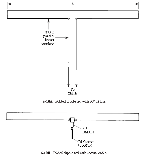
Figure 6-10A shows the folded dipole antenna. This antenna basically consists of two half-wavelength conductors shorted together at the ends and fed in the mid-dle of one of them. The folded dipole is most often built from 300-Ωtelevision an-tenna twin-lead transmission line. Because the feedpoint impedance is nearly 300 Ω,the same type of twin lead can also be used for the transmission line. The folded di-pole will exhibit excellent wide-bandwidth properties, especially on the lower bands.A disadvantage of this form of antenna is that the transmitter has to match the300-Ω balanced transmission line. Unfortunately, most modern radio transmitters are designed to feed coaxial-cable transmission line. Although an antenna tuner can be placed at the transmitter end of the feedline, it is also possible to use a 4:1 balun transformer at the feedpoint (Fig. 6-10B).

This arrangement makes the folded dipolea reasonable match to 52- or 75-Ω coaxial-cable transmission line.Another method for broadbanding the dipole is to use two identical dipoles fedfrom the same transmission line, and arranged to form a “bowtie” as shown in Fig. 6-11.The use of two identical dipole elements on each side of the transmission line has theeffect of increasing the conductor cross sectional area so that the antenna has a slightly improved length/diameter ratio.The bowtie dipole was popular in the 1930s and 1940s, and became the basis for the earliest television receiver antennas (TV signals are 3 to 5 MHz wide, so they requirea broadbanded antenna). It was also popular during the 1950s as the so-called Wonder Bar antenna for 10 m. It still finds use, but it has faded somewhat in popularity.The cage dipole(Fig. 6-12) is similar in concept, if not construction, to the bowtie. Again, the idea is to connect several parallel dipoles together from the same transmission line in an effort to increase the apparent cross-sectional area. In thecase of the cage dipole, however, spreader disk insulators are constructed to keepthe wires separated. The insulators can be built from plexiglass, lucite, or ceramic.
They can also be constructed of materials such as wood, if the wood is properlytreated with varnish, polyurethene, or some other material that prevents it from be-coming waterlogged. The spreader disks are held in place with wire jumpers (see in-set to Fig. 6-12) that are soldered to the main element wires.A tactic used by some builders of both bowtie and cage dipoles is to make the el-ements slightly different lengths. This “stagger tuning” method forces one dipole tofavor the upper end of the band, and the other to favor the lower end of the band.The overall result is a slightly flatter frequency response characteristic across theentire band. On the cage dipole, with four half-wavelength elements, it should bepossible to overlap even narrower sections of the band in order to create an evenflatter characteristic.
Subscribe to:
Comments (Atom)