Troubleshooting TV Reception Problems

Be aware of reception blockers , such long range distance from tv tower stations 


1. Distance from Tower

Use Directionl/omnidirectional  antenna with high gain 


Monopole Antenna

Monopole Antenna - The operating principle of rod antennas (or monopoles) is based on the fact that the current distribution on an antenna structure that is only a quarter wavelength long is identical to that on a half-wave dipole if the antenna element "missing" from the dipole is replaced by a highly conducting surface. As a result of this reflection principle , vertical quarter-wave antennas on conducting ground have basically the same radiation pattern as half-wave dipole antennas. There is of course no radiation into the shadowed half of the space. The input impedance is half that of a dipole, exhibiting values between approx. 30 Ω and 40 Ω.

The conducting surface on which the monopole is erected plays an important part in enabling the reflection principle to take effect. Even on reasonably conducting ground (such as a field of wet grass) and particularly on poorly conducting ground (dry sand) it is usual and helpful to put out a ground net of wires (commonly also called radials).
Figure below shows the influence of ground conductivity on the vertical pattern of a monopole antenna:
 

A special form of a monopole antenna is the so called groundplane antenna as figure below. It is characterized by several wires or rods (known as radials) which are arranged in a radial configuration from the feed point under a certain angle. Typically an angle of approx. 135° to the quarter wave monopole is used in order to increase the feed point resistance to a value of approx. 50 Ω which can easily be matched to commonly used coaxial cables.
 
Groundplane antennas are used as vertically polarized omnidirectional antennas even in the VHF/UHF frequency range.

Free Space

Free space conditions require a direct line of sight between the two antennas involved.
Consequently no obstacles must reach into the path between them. Furthermore in order to avoid the majority of effects caused by superposition of direct and reflected signals, it is necessary that the first Fresnel ellipsoid is completely free of obstacles :
 
 
Free Fresnel Ellipsoid

The first Fresnel ellipsoid is defined as a rotational ellipsoid with the two antennas at its focal points. Within this ellipsoid the phase difference between two potential paths is less than half a wavelength. 
The radius (b) at the center of the ellipsoid can be calculated based on the formula:
where b is the radius in m,
d is the distance between RX and TX in km,

and f is the frequency in GHz.
 

Antenna Gain

Antenna Gain - While the gain definition assumes ideal matching between the antenna and the connected cable and receiver or transmitter, in practice this is rarely the case. So what is measured in a non-ideally matched setup is called the practical gain of an antenna. The gain can be determined from the practical gain with the following formula:

where the amount of mismatch is expressed by the magnitude of the reflection coefficient r. 
 
Corresponding to the directivity factor, the gain G is the ratio of the radiation intensity Fmax obtained in the main direction of radiation to the radiation intensity Fi0, that would be generated by a loss-free isotropic radiator with the same input power Pt0.
 
 
In contrast to the directivity factor, the antenna efficiency η is taken into account in the above equation since the following applies:
For an antenna with efficiency η = 100%, this means that gain and directivity are equal.
In practice this is hardly the case, so the gain, which can be easily determined during measurements, is the parameter which is more frequently used.

Gain and directivity are often expressed in logarithmic form:

Contrary to common rules and standards, it is well established practice to indicate the reference with an additional letter after dB:
ı dBi refers to the isotropic radiator

ı dBd refers to the half-wave dipole

For example the following conversion applies: 0 dBd 2.15 dBi.


Maxwell Equation's

Maxwell's Equations - The equations postulated by the Scottish physicist James Clerk Maxwell in 1864 in his article A Dynamic Theory of the Electromagnetic Field are the foundations of classical electrodynamics, classical optics and electric circuits. This set of partial differential equations describes how electric and magnetic fields are generated and altered by each other and by the influence of charges or currents. Maxwell's equations represent one of the most elegant and concise ways to state the fundamentals of electricity and magnetism. From them one can develop most of the working relationships in the field. Because of their concise statement, they embody a high level of mathematical sophistication and are therefore not generally introduced in an introductory treatment of the subject, except perhaps as summary relationships.
These basic equations of electricity and magnetism can be used as a starting point for advanced courses, but are usually first encountered as unifying equations after the study of electrical and magnetic phenomena.


where rot (or curl) is a vector operator that describes the rotation of a three- dimensional vector field,


Equation (1) is Ampere's law. It basically states that any change of the electric field over time causes a magnetic field. Equation (2) is Faraday's law of induction, which describes that any change of the magnetic field over time causes an electric field. The other two equations relate to Gauss's law. (3) states that any magnetic field is solenoid and (4) defines that the displacement current through a surface is equal to the encapsulated charge.
From Maxwell's equations and the so called material equations
it is possible to derive a second order differential equation known as the telegraph equation:
where 𝜀 is the permittivity of a dielectric medium,
          𝜎 is the electrical conductivity of a material,
          𝜇 is the permeability of a material and
        
If one assumes that the conductivity of the medium in which a wave propagates is very small (𝜎 → 0) and if one limits all signals to sinusoidal signals with an angular frequency ω, the so called wave equation can be derived:
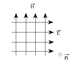
The simplest solution to this equation is known as a plane wave propagating in loss free homogenous space. For this wave, the following condition applies:
The vectors of the electric and magnetic field strength are perpendicular to each other and mutually also to the direction of propagation , see figure below.
Consequently the electric and magnetic field strengths are connected to each other via the so called impedance of free space:
Plan wave Description

Reference : Antenna Basic - Rohde & Schwarz