ground, and being fed in the center by coaxial cable. Some of the same comments asobtained for the inverted-vee antenna also apply to the sloping dipole, so please see that section also.Some operators like to arrange four sloping dipoles from the same mast suchthat they point in different directions around the compass (Fig. 6-9). A single four-position coaxial cable switch will allow switching a directional beam around the com-pass to favor various places in the world.
Antenna Handbook : Complete free tutorial antennas design , diy antenna , booster antenna, filter antenna , software antenna , free practical antenna book download !
Sloping dipole (“sloper” or “slipole”)
The sloping dipole(Fig. 6-8) is popular with those operators who need a low angle of radiation, and are not overburdened with a large amount of land to install the antenna. This antenna is also called the sloper and the slipole in various texts. The author prefers the term “slipole,” in order to distinguish this antenna from a sloping vertical of the same name. Whatever it is called, however, it is a half-wavelength di-pole that is built with one end at the top of a support, and the other end close to the
ground, and being fed in the center by coaxial cable. Some of the same comments asobtained for the inverted-vee antenna also apply to the sloping dipole, so please see that section also.Some operators like to arrange four sloping dipoles from the same mast suchthat they point in different directions around the compass (Fig. 6-9). A single four-position coaxial cable switch will allow switching a directional beam around the com-pass to favor various places in the world.
Transmission line responses
In order to understand the operation of transmission lines, we need to consider two cases:step-function response and the steady-state ac response. The step-function case involves a single event when a voltage at the input of the line snaps from zero(or a steady value) to a new (or nonzero) value, and remains there until all action dies out. This response tells us something of the behavior of pulses in the line, and infact is used to describe the response to a single-pulse stimulus. The steady-state ac response tells us something of the behavior of the line under stimulation by a sinusoidal RF signal.
Step-function response of a transmission line
Figure 3-3 shows a parallel transmission line with characteristic impedance Zo connected to a load impedance ZL. The generator at the input of the line consists of a voltage source Vin series with a source impedance Zs and a switch S1. Assume for the present that all impedances are pure resistances (i.e., R+j0). Also, assume that Zs=Zo.When the switch is closed at time To(Fig. 3-4A), the voltage at the input of theline (Vin) jumps to V/2. In Fig. 3-2, you may have noticed that the LC circuit resem-bles a delay line circuit. As might be expected, therefore, the voltage wave front propagates along the line at a velocity v of,
where v is the velocity, in meters per second L is the inductance, in henrys C is the capacitance, in farads
Inverted-vee dipole Antenna
The inverted-vee dipole is a half-wavelength antenna fed in the center like a dipole.By the rigorous definition, the inverted-vee is merely a variation on the dipoletheme. But in this form of antenna (Fig. 6-7), the center is elevated as high as possi-ble from the earth’s surface, but the ends droop to very close to the surface. Angle acan be almost anything convenient, provided that a> 90 degrees; typically, most in-verted-vee antennas use an angle of about 120 degrees. Although essentially a com-pensation antenna for use when the dipole is not practical, many operators believethat it is essentially a better performer on 40 and 80 m in cases where the dipole can-not be mounted at a half-wavelength (64 ft or so).By sloping the antenna elements down from the horizontal to an angle (as shownin Fig. 6-7), the resonant frequency is effectively lowered. Thus, the antenna will
need to be shorter for any given frequency than a dipole. There is no absolutely rig-orous equation for calculation of the overall length of the antenna elements. Al-though the concept of “absolute” length does not hold for regular dipoles, it is evenless viable for the inverted-vee. There is, however, a rule of thumb that can be fol-lowed for a starting point: Make the antenna about 6 percent shorter than a dipolefor the same frequency. The initial cut of the antenna element lengths (each quarter wavelength) is
After this length is determined, the actual length is found from the same cut-and-try method used to tune the dipole in the previous section.Bending the elements downward also changes the feedpoint impedance of theantenna and narrows its bandwidth. Thus, some adjustment in these departments isin order. You might want to use an impedance matching scheme at the feedpoint, oran antenna tuner at the transmitter.
High-frequency dipole antennas
Dipole Antenna: What is it? (And the Types of Antennas) -
What is a Dipole Antennas?
A dipole antenna (also known as a doublet or dipole aerial) is defined as a type of RF (Radio Frequency) antenna, consisting of two conductive elements such as rods or wires. The dipole is any one of the varieties of antenna that produce a radiation pattern approximating that of an elementary electric dipole. Dipole antennas are the simplest and most widely used type of antenna.
A ‘dipole’ means ‘two poles’ hence the dipole antenna consists of two identical conductive elements such as rods or metal wires. The length of the metal wires is approximately half of the maximum wavelength (i.e.,= Lambda/2) in free space at the frequency of operation.
In a perfect antenna, that is self-supported many wavelengths away from any ob-ject, Eq. 6.1 will yield the physical length. But in real antennas, the length calculated
above is too long. The average physical length is shortened by up to about 5 percentbecause of the velocity factor of the wire and capacitive effects of the end insulators.A more nearly correct approximation(remember that word, it's important) of ahalf-wavelength antenna is
where
L is the length of a half-wavelength radiator, in feet
FMHz is the operating frequency, in megahertz
ExampleCalculate the approximate physical length for a half-wavelength di-pole operating on a frequency of 7.25 MHz.
Solution :
or, restated another way:
It is unfortunate that a lot of people accept Eq. 6.2 as a universal truth, a kind ofimmutable law of The Universe. Perhaps abetted by books and articles on antennasthat fail to reveal the full story, too many people install dipoles without regard for reality. The issue is resonance. An antenna is a complex RLCnetwork. At some fre-quency, it will appear like an inductive reactance (X= +jXL), and at others it will appear like a capacitive reactance (X=–jXC). At a specific frequency, the reac-tances are equal in magnitude, but opposite in sense, so they cancel each other out:XL–XC= 0. At this frequency, the impedance is purely resistive, and the antenna issaid to be resonant.The goal in erecting a dipole is to make the antenna resonant at a frequency that isinside the band of interest, and preferably in the portion of the band most often used bythe particular station. Some of the implications of this goal are covered later on, but forthe present, assume that the builder will have to custom-tailor the length of the an-tenna. Depending on several local factors (among them, nearby objects, the shape ofthe antenna conductor, and the length/diameter ratio of the conductor) it might provenecessary to add, or trim, the length a small amount to reach resonance.
Reference:Practical Antenna Handbook -Joseph Carr
Transmission line characteristics
Velocity factor
In the section preceding this section, we discovered that the velocity of the wave (orsignal) in the transmission line is less than the free-space velocity (i.e., less than thespeed of light). Further, we discovered in Eq. 3.3 that velocity is related to the di-electric constant of the insulating material that separates the conductors in thetransmission line. Velocity factor vis usually specified as a decimal fraction of c,the speed of light (3 ×10⁸m/s). For example, if the velocity factor of a transmissionline is rated at “0.66,” then the velocity of the wave is 0.66c, or (0.66) (3 ×10⁸m/s)= 1.98 ×10⁸m/s.Velocity factor becomes important when designing things like transmission linetransformers, or any other device in which the length of the line is important. In mostcases, the transmission line length is specified in terms of electrical length, whichcan be either an angular measurement (e.g., 180° orπradians), or a relative measurekeyed to wavelength (e.g., one-half wavelength, which is the same as 180°). Thephysical lengthof the line is longer than the equivalent electrical length. For exam-ple, let’s consider a 1-GHz half-wavelength transmission line.A rule of thumb tells us that the length of a wave (in meters) in free space is 0.30/F,where frequencyFis expressed in gigahertz; therefore, a half-wavelength line is 0.15/F
At 1 GHz, the line must be 0.15 m/1 GHz = 0.15 m. If the velocity factor is 0.80, then thephysical lengthof the transmission line that will achieve the desired electrical lengthis [(0.15 m) (v)]/F= [(0.15 m) (0.80)]/1 GHz = 0.12 m. The derivation of the rule ofthumb is “left as an exercise for the student.” (Hint: It comes from the relationship be-tween wavelength, frequency, and velocity of propagation for any form of wave.)There are certain practical considerations regarding velocity factor that resultfrom the fact that the physical and electrical lengths are not equal. For example, ina certain type of phased-array antenna design, radiating elements are spaced a half-wavelength apart, and must be fed 180° (half-wave) out of phase with each other.The simplest interconnect is to use a half-wave transmission line between the 0°element and the 180° element. According to the standard wisdom, the transmissionline will create the 180° phase delay required for the correct operation of the an-tenna. Unfortunately, because of the velocity factor, the physical length for a one-half electrical wavelength cable is shorter than the free-space half-wave distancebetween elements. In other words, the cable will be too short to reach between theradiating elements by the amount of the velocity factor!Clearly, velocity factor is a topic that must be understood before transmissionlines can be used in practical situations. Table 3-1 shows the velocity factors for sev-eral types of popular transmission line. Because these are nominal values, the actualvelocity factor for any given line should be measured.
Transmission line noise
Transmission lines are capable of generating noise and spurious voltages that areseen by the system as valid signals. Several such sources exist. One source is thecoupling between noise currents flowing in the outer conductor and the inner con-ductor. Such currents are induced by nearby electromagnetic interference and othersources (e.g., connection to a noisy groundplane). Although coaxial design reducesnoise pickup, compared with parallel line, the potential for EMI exists. Selection ofhigh-grade line, with a high degree of shielding, reduces the problem.Another source of noise is thermal noises in the resistances and conductances.This type of noise is proportional to resistance and temperature.
There is also noise created by mechanical movement of the cable. One speciesresults from the movement of the dielectric against the two conductors. This form ofnoise is caused by electrostatic discharges in much the same manner as the sparkcreated by rubbing a piece of plastic against woolen cloth.A second species of mechanically generated noise is piezoelectricityin the di-electric. Although more common in cheap cables, one should be aware of it. Me-chanical deformation of the dielectric causes electrical potentials to be generated.Both species of mechanically generated noise can be reduced or eliminated byproper mounting of the cable. Although rarely a problem at lower frequencies, suchnoise can be significant at microwave frequencies when signals are low.
Coaxial cable capacitance
A coaxial transmission line possesses a certain capacitance per unit of length. This capacitance is defined by :
A long run of coaxial cable can build up a large capacitance. For example, acommon type of coax is rated at 65 pF/m. A 150-m roll thus has a capacitance of 65 pF/m ×(150 m), or 9750 pF. When charged with a high voltage, as is done inbreakdown voltage tests at the factory, the cable acts like a charged high-voltagecapacitor. Although rarely (if ever) lethal to humans, the stored voltage in newcable can deliver a nasty electrical shock and can irreparably damage electronic components.
Coaxial cable cutoff frequency Fo
The normal mode in which a coaxial cable propagates a signal is as a transverseelectromagnetic (TEM) wave, but others are possible—and usually undesirable.There is a maximum frequency above which TEM propagation becomes a prob-lem, and higher modes dominate. Coaxial cable should notbe used above a fre-quency of
where
F is the TEM-mode cutoff frequency
D is the diameter of the outer conductor, in inchesdis the diameter of the inner conductor, in inches
e is the dielectric constant
When maximum operating frequencies for cable are listed, it is the TEM modethat is cited. Beware of attenuation, however, when making selections for microwavefrequencies. A particular cable may have a sufficiently high TEM-mode frequency,but still exhibit a high attenuation per unit length at X or Ku bands.
(from Practical Antenna :by Joseph Carr) If you wantget hardcopy of this Practical Antenna Theory ,You canbuy this book :Practical Antenna Handbook by Joseph Carr:
Transmission line characteristic impedance (Zo)
The transmission line is an RLC network (see Fig. 3-2), so it has a characteristic impedance Zo, also sometimes called a surge impedance. Network analysis will show that Zo is a function of the per unit of length parameters resistance R,con-ductance G,inductance L, and capacitance C, and is found from equation :
where Zo is the characteristic impedance, in ohms
R is the resistance per unit length, in ohms
G is the conductance per unit length, in mhos
L is the inductance per unit length, in henrys
C is the capacitance per unit length, in farads
ω is the angular frequency in radians per second (2πF)
In microwave systems the resistances are typically very low compared with the reactances, so Eq. 3.1 can be reduced to the simplified form:
Example 3-1A nearly lossless transmission line (Ris very small) has a unit length inductance of 3.75 nH and a unit length capacitance of 1.5 pF. Find the char-acteristic impedance Zo,
Solution:
The characteristic impedance for a specific type of line is a function of the con-ductor size, the conductor spacing, the conductor geometry (see again Fig. 3-1), andthe dielectric constant of the insulating material used between the conductors. Thedielectric constant eis equal to the reciprocal of the velocity (squared) of the wavewhen a specific medium is used
In practical situations, we usually don’t need to calculate the characteristic im-pedance of a stripline, but rather design the line to fit a specific system impedance(e.g., 50 Ω). We can make some choices of printed circuit material (hence dielectricconstant) and thickness, but even these are usually limited in practice by the avail-ability of standardized boards. Thus, stripline widthis the variable parameter. Equa-tion 3.2 can be arranged to the form:

where Zo is the characteristic impedance, in ohms
R is the resistance per unit length, in ohms
G is the conductance per unit length, in mhos
L is the inductance per unit length, in henrys
C is the capacitance per unit length, in farads
ω is the angular frequency in radians per second (2πF)
In microwave systems the resistances are typically very low compared with the reactances, so Eq. 3.1 can be reduced to the simplified form:
Example 3-1A nearly lossless transmission line (Ris very small) has a unit length inductance of 3.75 nH and a unit length capacitance of 1.5 pF. Find the char-acteristic impedance Zo,
Solution:
where e is the dielectric constant (for a perfect vacuum e= 1.000) v is the velocity of the wave in the medium
(a)Parallel line
where Zo is the characteristic impedance, in ohms e is the dielectric constant S is the center-to-center spacing of the conductors d is the diameter of the conductors
(b) Coaxial line
where D is the diameter of the outer conductor d is the diameter of the inner conductor
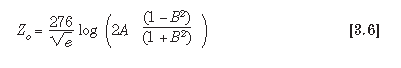
(c)Shielded parallel line
where A=s/d
B=s/D
(d)Stripline
where
et ,is the relative dielectric constant of the printed wiring board (PWB)
T is the thickness of the printed wiring board
W is the width of the stripline conductor
The relative dielectric constant e tused above differs from the normal dielectric constant of the material used in the PWB. The relative and normal dielectric con-stants move closer together for larger values of the ratio W/T.Example 3-2A stripline transmission line is built on a 4-mm-thick printed wiring board that has a relative dielectric constant of 5.5. Calculate the characteris-tic impedance if the width of the strip is 2 mm.
Solution :
In practical situations, we usually don’t need to calculate the characteristic im-pedance of a stripline, but rather design the line to fit a specific system impedance(e.g., 50 Ω). We can make some choices of printed circuit material (hence dielectricconstant) and thickness, but even these are usually limited in practice by the avail-ability of standardized boards. Thus, stripline widthis the variable parameter. Equa-tion 3.2 can be arranged to the form:
The impedance of 50 Ωis accepted as standard for RF systems, except in the cable TV industry. The reason for this diversity is that power handling ability and lowloss operation don’t occur at the same characteristic impedance. For example, the maximum power handling ability for coaxial cables occurs at 30 Ω, while the lowest loss occurs at 77 Ω; 50 Ωis therefore a reasonable tradeoff between the two points.In the cable TV industry, however, the RF power levels are minuscule, but lines arelong. The tradeoff for TV is to use 75 Ωas the standard system impedance in orderto take advantage of the reduced attenuation factor.
If you want get hardcopy of this Practical Antenna Theory ,You canbuy this book :Practical Antenna Handbook by Joseph Carr:
Subscribe to:
Comments (Atom)