Antenna Gain

Antenna Gain - While the gain definition assumes ideal matching between the antenna and the connected cable and receiver or transmitter, in practice this is rarely the case. So what is measured in a non-ideally matched setup is called the practical gain of an antenna. The gain can be determined from the practical gain with the following formula:

where the amount of mismatch is expressed by the magnitude of the reflection coefficient r. 

 

Corresponding to the directivity factor, the gain G is the ratio of the radiation intensity Fmax obtained in the main direction of radiation to the radiation intensity Fi0, that would be generated by a loss-free isotropic radiator with the same input power Pt0.

 

 

In contrast to the directivity factor, the antenna efficiency η is taken into account in the above equation since the following applies:

For an antenna with efficiency η = 100%, this means that gain and directivity are equal.
In practice this is hardly the case, so the gain, which can be easily determined during measurements, is the parameter which is more frequently used.
Gain and directivity are often expressed in logarithmic form:

Contrary to common rules and standards, it is well established practice to indicate the reference with an additional letter after dB:
ı dBi refers to the isotropic radiator
ı dBd refers to the half-wave dipole
For example the following conversion applies: 0 dBd ≈ 2.15 dBi. 

Reference:https://scdn.rohde-schwarz.com/ur/pws/dl_downloads/premiumdownloads/premium_dl_brochures_and_datasheets/premium_dl_whitepaper/Antenna_Basics_8GE01_1e.pdf

 

Maxwell Equation's

Maxwell's Equations - The equations postulated by the Scottish physicist James Clerk Maxwell in 1864 in his article A Dynamic Theory of the Electromagnetic Field are the foundations of classical electrodynamics, classical optics and electric circuits. This set of partial differential equations describes how electric and magnetic fields are generated and altered by each other and by the influence of charges or currents. Maxwell's equations represent one of the most elegant and concise ways to state the fundamentals of electricity and magnetism. From them one can develop most of the working relationships in the field. Because of their concise statement, they embody a high level of mathematical sophistication and are therefore not generally introduced in an introductory treatment of the subject, except perhaps as summary relationships.

These basic equations of electricity and magnetism can be used as a starting point for advanced courses, but are usually first encountered as unifying equations after the study of electrical and magnetic phenomena.

where rot (or curl) is a vector operator that describes the rotation of a three- dimensional vector field,

Equation (1) is Ampere's law. It basically states that any change of the electric field over time causes a magnetic field. Equation (2) is Faraday's law of induction, which describes that any change of the magnetic field over time causes an electric field. The other two equations relate to Gauss's law. (3) states that any magnetic field is solenoid and (4) defines that the displacement current through a surface is equal to the encapsulated charge.

From Maxwell's equations and the so called material equations

it is possible to derive a second order differential equation known as the telegraph equation:

where 𝜀 is the permittivity of a dielectric medium,

          𝜎 is the electrical conductivity of a material,

          𝜇 is the permeability of a material and

        

If one assumes that the conductivity of the medium in which a wave propagates is very small (𝜎 → 0) and if one limits all signals to sinusoidal signals with an angular frequency ω, the so called wave equation can be derived:

The simplest solution to this equation is known as a plane wave propagating in loss free homogenous space. For this wave, the following condition applies:

The vectors of the electric and magnetic field strength are perpendicular to each other and mutually also to the direction of propagation , see figure below.

Consequently the electric and magnetic field strengths are connected to each other via the so called impedance of free space:

Plan wave Description

Reference : Antenna Basic - Rohde & Schwarz

Radiation Pattern

The three-dimensional radiation behavior of antennas is described by their radiation pattern (normally in the far field). As explained before, only an isotropic radiator would exhibit the same radiation in every spatial direction, but this radiator cannot be implemented for any specified polarization and is therefore mainly suitable as a model and comparison standard. 

Dipoles and monopoles possess directivity. An electrically short dipole in free space has a three-dimensional radiation pattern shown in Figure below with nulls in the direction of the antenna's axis.

While the radiation pattern is actually three-dimensional, it is common however to describe this behavior with two planar patterns, also called the principal plane patterns. They can be obtained from the spatial radiation characteristics by looking at a cut-plane - usually through the origin and the maximum of radiation. Spherical coordinates as shown in Figure below are commonly used to describe a location in the three-dimensional space.

The horizontal pattern (see Figure below) shows the field strength as a function of the azimuth angle ϕ with a fixed ϑ (usually ϑ = 90°).

The vertical pattern (see Figure below) shows the field strength as a function of ϑ for a fixed ϕ (usually ϕ = +/- 90 ° or 0°/180°)

Usually antenna patterns are shown as plots in polar coordinates. This has the advantage that the radiation into all possible directions can quickly be visualized. In some occasions (i.e. for highly directive antennas) it can also be beneficial to plot the radiation pattern in Cartesian coordinates - because this reveals more details of the main beam and adjacent side lobes, see figure below.

From the radiation pattern the following additional parameters can be derived (see Figure below)

• The side lobe suppression (or side lobe level) is a measure of the relation between the main lobe and the highest side lobe.
• The half-power beamwidth (HPBW) is the angle between the two points in the main lobe of an antenna pattern that are down from the maximum by 3 dB. It is usually defined for both principal plane patterns.
• The front-to-back ratio specifies the level of radiation from the back of a directional antenna. It is the ratio of the peak gain in forward direction to the gain in the reverse (180°) direction. It is usually expressed in dB.

Reference : Antenna Basic - Rohde & Schwarz

Log Periodic Antenna

Antenna Theory - Log-periodic antenna - The Yagi-Uda antenna is mostly used for long time . However, for better reception  and to tune over a range of frequencies, we need to have another antenna known as the Log-periodic antenna. A Log-periodic antenna with good impedance is a logarithamically periodic function of frequency. 

A special type of directional antenna is the log-periodic dipole antenna (LPDA), where beam shaping is performed by means of several driven elements. The Log Periodic Dipole Antenna is made up of a number of parallel dipoles of increasing lengths and spacing (see Figure 26). Each dipole is fed out of phase to the element on either side by a common feed line. The angle α formed by the lines joining the dipole ends and by the longitudinal axis of the antenna remains constant, as well as the graduation factor 𝜏 which is equal to the ratio of the lengths of neighboring elements and their spacing: 

Log Periodic Dipole Antenna Design (courtesy Rohde & Schwarz)

This antenna type is characterized by its active and passive regions. The antenna is fed starting at the front (i.e. with the shortest dipole). The electromagnetic wave passes along the feed line and all dipoles that are markedly shorter than half a wavelength will not contribute to the radiation. 

The dipoles in the order of half a wavelength are brought into resonance and form the active region, which radiates the electromagnetic wave back into the direction of the shorter dipoles. 

This means that the longer dipoles located behind this active region are not reached by the electromagnetic wave at all. The active region usually comprises of 3 to 5 dipoles and its location obviously varies with frequency. The lengths of the shortest and longest dipoles of an LPDA-Log Periodic Dipole Antenna determine the maximum and minimum frequencies at which it can be used.

Due to the fact that at a certain frequency only some of the dipoles contribute to the radiation, the directivity (and therefore also the gain) that can be achieved with LPDAs-Log Periodic Dipole Antenna is relatively small in relation to the overall size of the antenna. However, the advantage of the LPDA is its large bandwidth which is - in theory - only limited by physical constraints.

The radiation pattern, of an LPDA is almost constant over the entire operating frequency range. In the H-plane it exhibits a half-power beamwidth of approx. 120°, while the E-plane pattern is typically 60° to 80° wide. The beamwidth in the H-plane can be reduced to values of approx. 65° by stacking two LPDAs in V-shape.

Example of a V-Stacked LPDA Antenna

V-stacked LPDA antennas have E- and H-plane patterns with very similar half power beamwidths. Additionally they feature approx. 1.5 dB more gain compared to a normal LPDA.

Radiation pattern of a V-stacked LPDA - E-plane (black), H-plane (blue)

Reference:https://scdn.rohde-schwarz.com/ur/pws/dl_downloads/premiumdownloads/premium_dl_brochures_and_datasheets/premium_

dl_whitepaper/Antenna_Basics_8GE01_1e.pdf

Antenna Impedance Measurement

Input Impedance 

One of the most significant parameters of an antenna is its input impedance: 

𝑍𝑖𝑛 = 𝑅𝑖𝑛 +𝑗𝑋𝑖𝑛 

This is the impedance present at the antenna feed point. Its real part Rin can be split up into the radiation resistance RR and the loss resistance RL 

𝑅𝑖𝑛 = 𝑅𝑅 + 𝑅𝐿 

It should be noted however that the radiation resistance, being the quotient of the radiated power and the square of the RMS value of the antenna current, is spatially dependent. This applies also to the antenna current itself. Consequently, when specifying the radiation resistance, its location on the antenna needs to be indicated.

Quite commonly the antenna feed point is specified, and equally often the current maximum. The two points coincide for some, but by no means for all types of antenna. The imaginary part Xin of the input impedance disappears if the antenna is operated at resonance. Electrically very short linear antennas have capacitive impedance values (Xin < 0), whereas electrically too long linear antennas can be recognized by their inductive imaginary part (Xin > 0).

Nominal Impedance The nominal impedance Zn is a mere reference quantity. It is commonly specified as the characteristic impedance of the antenna cable, to which the antenna impedance must be matched (as a rule Zn = 50 Ω). 

Impedance Matching and VSWR If the impedance of an antenna is not equal to the impedance of the cable and/or the impedance of the transmitter, a certain discontinuity occurs. The effect of this discontinuity is best described for the transmit case, where a part of the power is reflected and consequently does not reach the antenna (see Figure below.) However the same will happen with the received power from the antenna that does not fully reach the receiver due to mismatch caused by the same discontinuity.

Forward and reflected power due to mismatch 

The amount of reflected power can be calculated based on the equivalent circuit diagram of a transmit antenna (see Figure below).

For optimum performance, the impedance of the transmitter (ZS) must be matched to the antenna input impedance Zin. According to the maximum power transfer theorem, maximum power can be transferred only if the impedance of the transmitter is a complex conjugate of the impedance of the antenna and vice versa. Thus the following condition for matching applies: 

𝑍𝑖𝑛 = 𝑍𝑆 ∗ 𝑤ℎ𝑒𝑟𝑒 𝑍𝑖𝑛 = 𝑅𝑖𝑛 + 𝑗𝑋𝑖𝑛 𝑎𝑛𝑑 𝑍𝑆 = 𝑅𝑆 + 𝑗𝑋𝑆 

If the condition for matching is not satisfied, then some power may be reflected back and this leads to the creation of standing waves, which are characterized by a parameter called Voltage Standing Wave Ratio (VSWR). 

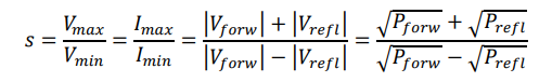
The VSWR is defined (as implicated by its name) as the ratio of the maximum and minimum voltages on a transmission line. However it is also possible to calculate VSWR from currents or power levels as the following formula shows: 

Another parameter closely related to the VSWR is the reflection coefficient r. It is defined as the ratio of the amplitude of the reflected wave Vrefl to the amplitude of the incident wave Vforw : 

It is furthermore related to the VSWR by the following formula: 

The return loss ar derives from the reflection coefficient as a logarithmic measure:

 

So there are in fact several physical parameters for describing the quality of impedance matching; these can simply be converted from one to the other as required. For easy conversion please refer to the table below: 

Baluns and Impedance Matching

An Antenna is normally connected to a transmission line and good matching between them is very important. A coaxial cable is often employed to connect an antenna mainly due to its good performance and low cost. A half-wavelength dipole antenna with impedance of about 73 ohms is widely used in practice. From the impedance -matching point, this dipole can match well with a 50 or 75 ohm standard coaxial cable . Now the question is : can we connect a coaxial cable directly to a dipole ?

As illustrated n figure below . when a dipole is directly connected to a coaxial cable, there is a proble: A part of the current comming from the outer conductor of the cable may go to the outside of the outer conductor at the end and return to the source rather than flow to the dipole .

A Dipole Antenna directly connected to coaxial cable 

 This undesirable current will make the cable become part of the antenna and radiate or receive unwated signal, which could be a very serious problem in some cases. In order to resolve this problem, a balun is required.

The term balun is an abbreviation of the two words balance and unbalance. It is a device that connects a balanced antenna ( a dipole , in this case) to an unbalanced transmission line (a  coaxial cable, where the inner conductor is not balanced with the outer conductor). The aim is to eliminate the undesirable current comming back on the outside of the cable. There are a few baluns developed for this important application. Figure below shows two examples . 

Two example of baluns

The sleeve balun is a very compact configuration: a metal tube of 1/4 Lambda is added to cable to form another transmission line (a coax again) with the outer conductor cable , and a short circuit is made at the base which produces an infinite impedance at the open top. The Leaky current is reflected back with a phase shift of 180 degrees, which results in the cancellation of the unwanted current on the outside of the cable. This balun is a narrowband device. If the short-circuit end is made as a sliding bar, it can be adjusted for a wide frequency range (but it is still a narrowband device). 

The second example is a ferrite-bead choke placed on the outside of the coaxial cable. It is widely used in EMC Industry and its function is to produce a high impedance, more precisely high inductance due to the large bandwidth may be obtained ( an octave or more). But this device is normally just suitable for frequencies below 1 GHz. which is determined by the ferrite properties it can be lossy, which can reduce the measured antenna efficiency.

Reference:https://scdn.rohde-schwarz.com/ur/pws/dl_downloads/premiumdownloads

/premium_dl_brochures_and_datasheets/premium_dl_whitepaper/Antenna_Basics_8GE01_1e.pdf