Free Space

Free space conditions require a direct line of sight between the two antennas involved.
Consequently no obstacles must reach into the path between them. Furthermore in order to avoid the majority of effects caused by superposition of direct and reflected signals, it is necessary that the first Fresnel ellipsoid is completely free of obstacles :

 

 

Free Fresnel Ellipsoid

The first Fresnel ellipsoid is defined as a rotational ellipsoid with the two antennas at its focal points. Within this ellipsoid the phase difference between two potential paths is less than half a wavelength. 

The radius (b) at the center of the ellipsoid can be calculated based on the formula:

where b is the radius in m,
d is the distance between RX and TX in km,
and f is the frequency in GHz.

 

Reference:https://scdn.rohde-schwarz.com/ur/pws/dl_downloads/premiumdownloads/premium_dl_brochures_and_datasheets/premium_dl_whitepaper/Antenna_Basics_8GE01_1e.pdf

Antenna Gain

Antenna Gain - While the gain definition assumes ideal matching between the antenna and the connected cable and receiver or transmitter, in practice this is rarely the case. So what is measured in a non-ideally matched setup is called the practical gain of an antenna. The gain can be determined from the practical gain with the following formula:

where the amount of mismatch is expressed by the magnitude of the reflection coefficient r. 

 

Corresponding to the directivity factor, the gain G is the ratio of the radiation intensity Fmax obtained in the main direction of radiation to the radiation intensity Fi0, that would be generated by a loss-free isotropic radiator with the same input power Pt0.

 

 

In contrast to the directivity factor, the antenna efficiency η is taken into account in the above equation since the following applies:

For an antenna with efficiency η = 100%, this means that gain and directivity are equal.
In practice this is hardly the case, so the gain, which can be easily determined during measurements, is the parameter which is more frequently used.
Gain and directivity are often expressed in logarithmic form:

Contrary to common rules and standards, it is well established practice to indicate the reference with an additional letter after dB:
ı dBi refers to the isotropic radiator
ı dBd refers to the half-wave dipole
For example the following conversion applies: 0 dBd ≈ 2.15 dBi. 

Reference:https://scdn.rohde-schwarz.com/ur/pws/dl_downloads/premiumdownloads/premium_dl_brochures_and_datasheets/premium_dl_whitepaper/Antenna_Basics_8GE01_1e.pdf

 

Maxwell Equation's

Maxwell's Equations - The equations postulated by the Scottish physicist James Clerk Maxwell in 1864 in his article A Dynamic Theory of the Electromagnetic Field are the foundations of classical electrodynamics, classical optics and electric circuits. This set of partial differential equations describes how electric and magnetic fields are generated and altered by each other and by the influence of charges or currents. Maxwell's equations represent one of the most elegant and concise ways to state the fundamentals of electricity and magnetism. From them one can develop most of the working relationships in the field. Because of their concise statement, they embody a high level of mathematical sophistication and are therefore not generally introduced in an introductory treatment of the subject, except perhaps as summary relationships.

These basic equations of electricity and magnetism can be used as a starting point for advanced courses, but are usually first encountered as unifying equations after the study of electrical and magnetic phenomena.

where rot (or curl) is a vector operator that describes the rotation of a three- dimensional vector field,

Equation (1) is Ampere's law. It basically states that any change of the electric field over time causes a magnetic field. Equation (2) is Faraday's law of induction, which describes that any change of the magnetic field over time causes an electric field. The other two equations relate to Gauss's law. (3) states that any magnetic field is solenoid and (4) defines that the displacement current through a surface is equal to the encapsulated charge.

From Maxwell's equations and the so called material equations

it is possible to derive a second order differential equation known as the telegraph equation:

where 𝜀 is the permittivity of a dielectric medium,

          𝜎 is the electrical conductivity of a material,

          𝜇 is the permeability of a material and

        

If one assumes that the conductivity of the medium in which a wave propagates is very small (𝜎 → 0) and if one limits all signals to sinusoidal signals with an angular frequency ω, the so called wave equation can be derived:

The simplest solution to this equation is known as a plane wave propagating in loss free homogenous space. For this wave, the following condition applies:

The vectors of the electric and magnetic field strength are perpendicular to each other and mutually also to the direction of propagation , see figure below.

Consequently the electric and magnetic field strengths are connected to each other via the so called impedance of free space:

Plan wave Description

Reference : Antenna Basic - Rohde & Schwarz

Radiation Pattern

The three-dimensional radiation behavior of antennas is described by their radiation pattern (normally in the far field). As explained before, only an isotropic radiator would exhibit the same radiation in every spatial direction, but this radiator cannot be implemented for any specified polarization and is therefore mainly suitable as a model and comparison standard. 

Dipoles and monopoles possess directivity. An electrically short dipole in free space has a three-dimensional radiation pattern shown in Figure below with nulls in the direction of the antenna's axis.

While the radiation pattern is actually three-dimensional, it is common however to describe this behavior with two planar patterns, also called the principal plane patterns. They can be obtained from the spatial radiation characteristics by looking at a cut-plane - usually through the origin and the maximum of radiation. Spherical coordinates as shown in Figure below are commonly used to describe a location in the three-dimensional space.

The horizontal pattern (see Figure below) shows the field strength as a function of the azimuth angle ϕ with a fixed ϑ (usually ϑ = 90°).

The vertical pattern (see Figure below) shows the field strength as a function of ϑ for a fixed ϕ (usually ϕ = +/- 90 ° or 0°/180°)

Usually antenna patterns are shown as plots in polar coordinates. This has the advantage that the radiation into all possible directions can quickly be visualized. In some occasions (i.e. for highly directive antennas) it can also be beneficial to plot the radiation pattern in Cartesian coordinates - because this reveals more details of the main beam and adjacent side lobes, see figure below.

From the radiation pattern the following additional parameters can be derived (see Figure below)

• The side lobe suppression (or side lobe level) is a measure of the relation between the main lobe and the highest side lobe.
• The half-power beamwidth (HPBW) is the angle between the two points in the main lobe of an antenna pattern that are down from the maximum by 3 dB. It is usually defined for both principal plane patterns.
• The front-to-back ratio specifies the level of radiation from the back of a directional antenna. It is the ratio of the peak gain in forward direction to the gain in the reverse (180°) direction. It is usually expressed in dB.

Reference : Antenna Basic - Rohde & Schwarz

Log Periodic Antenna

Antenna Theory - Log-periodic antenna - The Yagi-Uda antenna is mostly used for long time . However, for better reception  and to tune over a range of frequencies, we need to have another antenna known as the Log-periodic antenna. A Log-periodic antenna with good impedance is a logarithamically periodic function of frequency. 

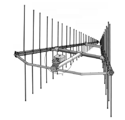
A special type of directional antenna is the log-periodic dipole antenna (LPDA), where beam shaping is performed by means of several driven elements. The Log Periodic Dipole Antenna is made up of a number of parallel dipoles of increasing lengths and spacing (see Figure 26). Each dipole is fed out of phase to the element on either side by a common feed line. The angle α formed by the lines joining the dipole ends and by the longitudinal axis of the antenna remains constant, as well as the graduation factor 𝜏 which is equal to the ratio of the lengths of neighboring elements and their spacing: 

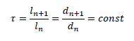
Log Periodic Dipole Antenna Design (courtesy Rohde & Schwarz)

This antenna type is characterized by its active and passive regions. The antenna is fed starting at the front (i.e. with the shortest dipole). The electromagnetic wave passes along the feed line and all dipoles that are markedly shorter than half a wavelength will not contribute to the radiation. 

The dipoles in the order of half a wavelength are brought into resonance and form the active region, which radiates the electromagnetic wave back into the direction of the shorter dipoles. 

This means that the longer dipoles located behind this active region are not reached by the electromagnetic wave at all. The active region usually comprises of 3 to 5 dipoles and its location obviously varies with frequency. The lengths of the shortest and longest dipoles of an LPDA-Log Periodic Dipole Antenna determine the maximum and minimum frequencies at which it can be used.

Due to the fact that at a certain frequency only some of the dipoles contribute to the radiation, the directivity (and therefore also the gain) that can be achieved with LPDAs-Log Periodic Dipole Antenna is relatively small in relation to the overall size of the antenna. However, the advantage of the LPDA is its large bandwidth which is - in theory - only limited by physical constraints.

The radiation pattern, of an LPDA is almost constant over the entire operating frequency range. In the H-plane it exhibits a half-power beamwidth of approx. 120°, while the E-plane pattern is typically 60° to 80° wide. The beamwidth in the H-plane can be reduced to values of approx. 65° by stacking two LPDAs in V-shape.

Example of a V-Stacked LPDA Antenna

V-stacked LPDA antennas have E- and H-plane patterns with very similar half power beamwidths. Additionally they feature approx. 1.5 dB more gain compared to a normal LPDA.

Radiation pattern of a V-stacked LPDA - E-plane (black), H-plane (blue)

Reference:https://scdn.rohde-schwarz.com/ur/pws/dl_downloads/premiumdownloads/premium_dl_brochures_and_datasheets/premium_

dl_whitepaper/Antenna_Basics_8GE01_1e.pdf