Large wire loop antennas

THERE ARE TWO BASIC FORMS OF LOOP ANTENNAS: SMALL AND LARGE. THESE TWO TYPES have different characteristics, work according to different principles, and have different purposes. Small loops are those in which the current flowing in the wire has the same phase and amplitude at every point in the loop (which fact implies a very short wire length, i.e., less than 0.2 ). Such loops respond to the magnetic field component of the electromagnetic radio wave. A large loop antenna has a wire length greater than 0.2 , with most being either /2, 1 , or 2 . The current in a large loop varies along the length of the wire in a manner similar to other wire antennas.

Lambda/2 large loops

 The performance of large wire loop antennas depends in part on their size. Figure 14-1 shows a half-wavelength loop (i.e., one in which the four sides are each /8 long). There are two basic configurations for this antenna: continuous (S1 closed) and open (S1 open). In both cases, the feedpoint is at the midpoint of the side opposite the switch. The direction of the main reception, or radiation lobe (i.e., the direction of maximum reception), depends on whether S1 is open or closed. With S1 closed, the main lobe is to the right (solid arrow); and with S1open, it is to the left (broken arrow). Direction reversal can be achieved by using a switch (or relay) at S1, although some people opt for unidirectional operation by eliminating S1, and leaving the loop either open or closed. The feedpoint impedance is considerably different in the two configurations. In the closed-loop situation (i.e., S1 closed), the antenna can be modeled as if it were a half-wavelength dipole bent into a square and fed at the ends. The feedpoint (X1 X2) impedance is on the order of 3 kΩ because it occurs at a voltage antinode (current node). The current antinode (i.e., Imax) is at S1, on the side opposite the feedpoint. An antenna tuning unit (ATU), or RF impedance transformer, must be used to match the lower impedance of the transmission lines needed to connect to receivers. The feedpoint impedance of the open-loop configuration (S1 open) is low because the current antinode occurs at X1 X2. Some texts list the impedance as “about 50 Ω,” but my own measurements on several test loops were somewhat higher (about 70 Ω). In either case, the open loop is a reasonable match for either 52- or 75-Ωcoaxial cable.

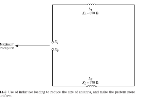
Neither Lambda/2 loop configuration shows gain over a dipole. The figure usually quoted is 1-dB forward gain (i.e., a loss compared with a dipole), and about 6-dB front-to-back ratio (FBR). Such low values of FBR indicate that there is no deep notch (“null”) in the pattern. A lossy antenna with a low FBR seems like a born loser, and in most cases it is. But the /2 loop finds a niche where size must be constrained, for one reason or another. In those cases, the /2 loop can be an alternative. These antennas can be considered limited-space designs, and can be mounted in an attic, or other limitedaccess place, as appropriate. A simple trick will change the gain, as well as the direction of radiation, of the closed version of the /2 loop. In Fig. 14-2, a pair of inductors (L1 and L2) are inserted into the circuit at the midpoints of the sides adjacent to the side containing the feedpoints. These inductors should have an inductive reactance XL of about 360 Ω in the center of the band of operation. The inductance of the coil is

The coils force the current antinodes toward the feedpoint, reversing the direction of the main lobe, and creating a gain of about 

1 dB over a half-wavelength dipole. The currents flowing in the antenna can be quite high, so when making the coils, be sure to use a size that is sufficient for the power and current levels anticipated. The 2- to 3-in B&W Air-Dux style coils are sufficient for most amateur radio use. Smaller coils are available on the market, but their use is limited to low-power situations.

Build Phasing Transformer Antenna

A directional antenna has the ability to enhance reception of desired signals, while rejecting undesired signals arriving from slightly different directions. Although directivity normally means a beam antenna, or at least a rotatable dipole, there are certain types of antenna that allow fixed antennas to be both directive and variable. See Chap. 7 for fixed but variable directional antennas and Chap. 11 for fixed and non-variable directive arrays. Those antennas are transmitting antennas, but they work equally well for reception. This section shows a crude, but often effective, directional antenna that allows one to select the direction of reception with pin plugs or switches.

Consider Fig. 13-10. In this case, a number of quarter-wavelength radiators are fanned out from a common feedpoint at various angles from the building. At the near end of each element is a female banana jack. A pair of balanced feedlines from the receiver (300-Ω twin lead, or similar) are brought to the area where the antenna elements terminate. Each wire in the twin lead has a banana plug attached. By selecting which banana jack is plugged into which banana plug, you can select the directional pattern of the antenna. If the receiver is equipped with a balanced antenna input, then simply connect the other end of the twin lead direction to the receiver. Otherwise, use one of the couplers shown in Fig. 13-11.

Figure 13-11A shows a balanced antenna coupler that is tuned to the frequency of reception. The coil is tuned to resonance by the interaction of the inductor and the capacitor. Antenna impedance is matched by selecting the taps on the inductor to which the feedline is attached. A simple RF broadband coupler is shown in Fig. 13-11B. This transformer is wound over a ferrite core, and consists of 12 to 24 turns of no. 26 enameled wire, with more turns being used for lower frequencies, and fewer for higher frequencies. Experiment with the number of turns in order to determine the correct value. Alternatively, use a 1:1 balun transformer instead of Fig. 13-11B; the type intended for amateur radio antennas is overkill powerwise, but it will work nicely.

The antenna of Fig. 13-10 works by phasing the elements so as to null, or enhance (as needed), certain directions. This operation becomes a little more flexible if you build a phasing transformer, as shown in Fig. 13-11C and 13-11D. Windings L1, L2, and L3 are wound “trifilar” style onto a ferrite core. Use 14 turns of no. 26 enameled wire for each winding. The idea in this circuit is to feed one element from coil L2 in the same way all of the time. This port becomes the 0° phase reference. The other port, B, is fed from a reversible winding, so it can either be in phase or 180°out of phase with port A. Adjust the DPDT switch and the banana plugs of Fig. 13-10 for the best reception.

Directional beam antennas

THE DIRECTIONAL BEAM ANTENNA DOES SEVERAL JOBS. FIRST, IT PROVIDES AN APPARENT increase in radiated power, because it focuses available transmitter power into a single (or at worst limited) direction.

For this reason, a bidirectional dipole has a gain of approximately 2 dB over an isotropic radiator. Add one or more additional elements, and the focusing becomes nearly unidirectional, which increases the effective radiated power (ERP) even more.

Second, the beam increases the received signal available at the inputs of the receiver. Antennas are generally reciprocal, so they will work for receiving as they do for transmitting. Finally, the directivity of the beam antenna allows the operator to null interfering stations. In fact, it is the last attribute of the beam that is most useful on today’s crowded bands.

All in all, if your funds are too little to provide both increased RF power and a good antenna system, then spend what is available on the antenna—not on the power. In this chapter we will focus on directional antennas that can be built relatively easily.

It is assumed that most readers who want a triband multielement Yagi will prefer to buy a commercial product, rather than build a homebrew model. The material herein concentrates on homebrew projects that are within the reach and capabilities of most readers. The first of these is not a beam antenna at all, but rather a rotatable dipole.

Rotatable dipole 

The dipole is a bidirectional antenna with a figure-8 pattern (when viewed from above). The dipole is a half-wavelength and is usually installed horizontally, although vertical half-wavelength dipoles are known. Although the length of the dipole is too great for rotatability at the lower bands, it is within reason for the higher band. For example, the size of the halfwave dipole is approximately 16 ft on 10 m and 22 ft on 15 m. Even the 33-ft length on 20 m is not unreasonable for amateur constructors. The length of the dipole is found from

This length is approximate because of end effects and other phenomena, so some “cut and try” is required. Example 12-1 Find the length of a dipole antenna for a frequency of 24.930 MHz in the 12-m amateur radio band. Solution:

The half-wave dipole is fed in the center by coaxial cable. Each element of the dipole is one-half of the overall length (or, in the example given, about 9.4 ft). Figure 12-1 shows a rotatable dipole that can be designed for use on 15, 12, and 10 m. The radiator elements are made from 10-ft lengths of 3⁄4-in aluminum tubing. The tubing is mounted on “beehive” standoff insulators, which in turn are mounted on a 4-ft length of 2 2 lumber. 

The lumber should be varnished against weathering. In a real pinch, the elements can be mounted directly to the lumber without the insulators, but this is not the recommended practice. The mast is attached to the 2 2 lumber through any of several means. 

The preferred method is the use of a 1-in pipe flange. These devices are available at hardware stores under the names floor flange and right-angle flange. The 10-ft lengths of pipe are the standard lengths available in hardware stores, so it was selected as being closest to the required 22 ft for 15 m. A 0.14-µH loading coil is used at the center, between the elements, in order to make up for the short length. The dimensions of the coil are 4 to 5 turns, 0.5-in diameter, 4-in length. For low power levels, the coil can be made of no. 10 (or no. 12) solid wire—and, for higher levels, 1⁄8-in copper tubing. There are two basic ways to feed the antenna, and these are shown in details A and B in Fig. 12-1. The traditional method is to connect the coaxial cable (in parallel) across the inductor. This method is shown in Fig. 12-1, detail A. 

A second method is to link couple the coil to the line through a one- to three-turn loop (as needed for impedance matching). This is the method that would be used for a toroidal inductor. Lower frequencies can be accommodated by changing the dimensions of the coil. The coil cannot be scaled, simply because the relative length of the antenna changes as the frequency changes. But it is possible to cut and try by adding turns to the coil, one turn at a time, and remeasuring the resonant frequency. 

Adding inductance to the coil will make the antenna usable on 17 m and 20 m, as well as on 15 m. Another method for building a rotatable dipole for lower frequencies is to increase the element lengths. On 17 m, the overall length is approximately 27.4 ft, so each element length is 13.7 ft long. This length can be achieved by either of two methods. First, adjacent sizes of aluminum tubing are designed so that the smaller will be a slip-fit inside of the larger. What constitutes “adjacent sizes” depends on the wall thickness, but for one common brand, the 7⁄8-in is adjacent to the 3⁄4-in size. 

You can use two smaller lengths to make the larger lengths of pipe, and cut it to size. This method is only available to those readers who have a commercial or industrial metals distributor nearby, because the 16-ft lengths are not generally available from hardware stores. Bands higher than 15 m (i.e., 12 and 10 m) can be accommodated by using the 10-ft lengths of tubing, but without the inductor. The tubing is cut to the desired half-wavelength size and used directly.

360 Degree Directional Array Antenna

The phased vertical antenna concept can be used to provide round-the-compass control of the antenna pattern. Figure 11-5A shows how three quarter-wavelength verticals (arranged in a triangle that is a half-wavelength on each side) can be used to provide either end-fire or broadside patterns from any pair (A-B, A-C, or B-C).

Any given antenna (A, B, or C) will be grounded, fed at 0°, or fed with 180°. The table in Fig. 11-5B shows the relative phasing for each direction that was labelled in Fig. 11-5A. Either manual phase changing or switch-operated phase changing can be used, although the latter is preferred for convenience. Some international showcase broadcasters use antenna arrays formed into two or more concentric circles of vertical elements, with one element at the center. Selection of elements and phasing determines directivity and gain.

Feeding Phased Array Antenna

The second variation, shown in Fig. 11-2B, supposedly produces a 180° phase shift between antenna A and antenna B, when length L3 is an electrical half-wavelength. According to a much-publicized theory, the system of Fig. 11-2B

ought to produce the pattern of Fig. 11-1B—yet experience shows this claim is false. It seems that there are several problems with the system in Fig. 11-2B.

First, coax has a property called velocity factor(VF), which is the fraction of the speed of light at which signals in the cable propagate. The VF is a decimal fraction on the order of 0.66 to 0.90, depending upon the type of coax used. Unfortunately, the physical spacing between A and B is a real half-wavelength (L3 = 492/F), but the cable length is shorter by the velocity factor [L3' = (VF × 492) /F].

Consider an example. A 15-m phased vertical antenna system will have two 11-ft radiators, spaced 22 ft apart (approximately, depending upon exact frequency). If we use foam coax, with VF = 0.80, the cable length is 0.8 × 22 ft, or 17.6 ft. In other words, despite lots of publicity, the cable won’t fit between the towers! Second, the patterns shown in Fig. 11-1 are dependent upon one condition: the antenna currents are equal. If both of them are the same impedance, and are fed from the same transmitter, then it is reasonable to assume that the currents are equal—right? No, wrong! What about coax loss? Because of normal coax loss, which increases at higher frequencies, the power available to antenna Bin Fig. 11-1B is less than the power available to antenna A. Thus, the pattern will be somewhat distorted, because the current produced in Bis less than the current in A, when they should be equal.

The first problem is sometimes fixed by using unequal lengths for cables L1 and L2 (Fig. 11-2A), and using it for the out-of-phase case. For example, if we make L1 one-quarter wavelength and L2 three-quarter wavelength (Fig. 11-2C), antenna A is fed with a 90° phase lag (relative to the tee connector signal), while antenna B is fed with a 270° phase shift. The result is still a 180° phase difference.

Unfortunately, we have not solved the current level problem, and may have actually made it worse by adding still more lossy cable to the system. There is still another problem that is generic to the whole class of phased verticals. Once installed, the pattern is fixed. This problem doesn’t bother most point-topoint commercial stations, or broadcasters, because they tend to transmit in only one direction. But amateurs are likely to need a rotatable pattern. Neither the antennas in Fig. 11-1A nor that in Fig. 11-1B is rotatable without a lot of effort—like changing the coax feeds, or physically digging up the verticals and repositioning them. Fortunately, there is a single solution to all three problems. Figure 11-3 shows a two-port phasing transformer made from a toroidal balun kit. Use the kind of kit that makes a 1:1 balun transformer. Although we are not making a balun, we will need enough wire to make three windings, and that is the normal case for 1:1 baluns. Amidon Associates and others make toroidal balun kits.

Wind the three coils in trifilar style, according to the kit instructions. The dots in Fig. 11-3 show the “sense” of the coils, and they are important for correct phasing; call one end the “dot end” and the other end the “plain end” to keep them separate. If the dot end of the first coil is connected to J3 (and the transmitter), then connect the dot end of the second coil to the 0° output (J1, which goes to antenna A). The third coil is connected to a DPDT RF relay or switch. In the position shown, S1 causes the antennas to be 180° out of phase. In the other position, the “sense” of the third coil is reversed, so the antennas are in phase. Another phasing method is shown in Fig. 11-4. In this scheme, two convenient, but equal, lengths of coaxial cable (L1 and L2) are used to carry RF power to the antennas. One segment (L1) is fed directly from the transmitter’s coaxial cable (L3), while the other is fed from a phasing switch. The phasing switch is used to either by

pass or insert a phase-shifting length of coaxial cable (L4). For 180° phasing use the following equation to find the length (L4):

where L is the length of L4, in feet VF is the velocity factor (a decimal fraction) FMHz is the operating frequency, in megahertz

Some people use a series of switches to select varying amounts of phasing shift from 45° to 270°. Such a switch allows them to select any number of other patterns for special situations.

Directional phased vertical antennas

THE VERTICAL ANTENNA IS A PERENNIAL FAVORITE WITH RADIO COMMUNICATIONS users. The vertical is either praised, or cursed, depending upon the luck of the owner. “DXability” is usually the criterion for judging the antenna’s quality. Some amateurs can’t get out of their backyards with a vertical, and they let everyone within earshot know that such and such a brand is no good. Yet, another person routinely works New Zealand or Australia on 15 m using exactly the same brand of vertical. The proper installation of vertical antennas is dealt with in another chapter, so, for the present, let’s look at another problem attributed to vertical antennas. That problem is that vertical antennas are omnidirectionalin the azimuth aspect; that is, they send out and receive equally well from all directions. Some people moan that this pattern dissipates their power, and gives them a weaker signal “out where it counts” (true). However, the main disadvantage of the omnidirectional pattern is noise (QRN and QRM). “QRN” is natural noise from thunderstorms and other sources. “QRM” is man-made noise, and can consist of other stations or the many assorted forms of electrical filth that pollute the airwaves. All forms of noise, however, have one thing in common: they are directional with respect to the station. In other words, if you could null signals coming from the direction of the noise source (or undesired station), you would be able to hear desired stations much better. A directional antenna performs this task, so let’s look at some vertically polarized directional antennas. Although most amateurs seem to think that the effective radiated power (ERP) increase that the directional antenna gives them is the real reason to own one, the main benefit is actually on receive. Think about it for a moment. With anywhere from 100 to 1500 W available, the increase or decrease in signal strength (due to the directivity of the antenna) results in a minimal difference on the receive end, especially during good DX conditions. If we rotate the directional pattern, to null out interference, then we usually find that the change in our signal strength perceived by the other guy is small; the S meter reading of the desired station is minimally affected; but the amplitude of the interference source is greatly attenuated! The overall effect is an apparent increase in the other guy’s signal, even though the S meter tells a slightly different story. The improvement of signal-to-noise ratio (SNR) is tremendously improved.

Directivity and phasing 

So, how does a vertical antenna owner get the benefit of directivity without the kilobuck investment that a beam or quad costs? The usual solution is to use phased verticals. AM broadcast stations, with more than one tower, are using this type of system (although for different reasons than hams). The idea is to place two or more antennas in close proximity and feed them at specific phase angles to produce a desired radiation pattern. A lot of material is available in the literature on phased vertical antenna systems, and it is far too much to be reproduced here. There are “standard patterns” dating from before World War II that are created with different spacings and different phase angles of feed current. In this chapter, we will consider only one system. Figure 11-1 shows the patterns for a pair of quarter-wavelength vertical antennas spaced a half-wavelength (180°) apart. Without getting into complex phase shifting networks, there are basically two phasings that are easily obtained: 0° (antennas in phase) and 180° (antennas out of phase with each other). When the two antennas (A and B) are fed in phase with equal currents (Fig. 111A), the radiation pattern (shown somewhat idealized here) is a bidirectional figure 8 that is directionally perpendicular to the line of centers between the two antennas; this pattern is called a broadsidepattern. A sharp null exists along the line of centers (A-B). When the antennas are fed out of phase with each other by 180° (Fig. 11-1B), the pattern rotates 90° (a quarter way around the compass) and now exhibits directivity along the line of the centers (A-B); this is the “end fire” pattern. The interference cancelling null is now perpendicular to line A-B. It should be apparent that you can select your directivity by selecting the phase angle of the feed currents in the two antennas. Figure 11-2 shows the two feeding

systems usually cited for in-phase (Fig. 11-2A) and out-of-phase (Fig. 11-2B) systems. Figure 11-2A shows the coax from the transmitter coming to a coax tee connector. From the connector to the antenna feedpoints are two lengths of coax (L1 and L2) that are equal to each other, and identical. Given the variation between coaxial cables, I suspect that it would work better if the two cables were not merely the same length (L1 = L2), but also that they came from the same roll. 

Shortened coil-loaded dipoles

The half-wavelength dipole is too long for some applications where real estate is at a premium. The solution for many operators is to use a coil-loaded shortened dipole such as shown in Fig. 6-13. A shortened dipole (i.e., one which is less than a halfwavelength) is capacitive reactance. There is no reason why the loading coil cannot be any point along the radiator, but in Figs. 6-13A and 6-13B they are placed at 0 percent and 50 percent of the element length, respectively. The reason for this procedure is that it makes the calculation of coil inductances easier, and it also represents the most common practice.

Figure 6-13C shows a table of inductive reactances as a function of the percentage of a half-wavelength, represented by the shortened radiator. It is likely that the percentage figure will be imposed on you by the situation, but the general rule is to pick the largest figure consistent with the available space. For example, suppose you have about 40 ft available for a 40-m antenna that normally needs about 65 ft for a half-wavelength. Because 39 ft is 60 percent of 65 ft, you could use this value as the design point for this antenna. Looking on the chart, a 60 percent antenna with the loading coils at the midpoint of each radiator element wants to see an inductive reactance of 700 Ω. You can rearrange the standard inductive reactance equation (XL = 6.28 FL) to the form

where LµH is the required inductance, in microhenrys F is the frequency, in hertz (Hz) XL is the inductive reactance calculated from the table in Fig. 6-13C.
Example 6-2 Calculate the inductance required for a 60 percent antenna operating on 7.25 MHz. The table requires a reactance of 700 Ωfor a loaded dipole with the coils in the center of each element (Fig. 6-15B). Solution:


The inductance calculated above is approximate, and it might have to be altered by cut-and-try methods. The loaded dipole antenna is a very sharply tuned antenna. Because of this fact, you must either confine operation to one segment of the band, or provide an antenna tuner to compensate for the sharpness of the bandwidth characteristic. However, efficiency drops, markedly, far from resonance even with a transmission line tuner. The function of the tuner is to overcome the bad effects on the transmitter, but it does not alter the basic problem. Only a variable inductor in the antenna will do that trick (at least one commercial loaded dipole once used a motor-driven inductor at the center feedpoint). Figures 6-13D and E show two methods for making a coil-loaded dipole antenna. Figure 6-13D shows a pair of commercially available loading coils especially designed for this purpose. The ones shown here are for 40 m, but other models are also available. The inductor shown in Fig. 6-13E is a section of commercial coil stock connected to a standard end or center insulator. No structural stress is assumed by the coil—all forces are applied to the insulator, which is designed to take it.

Inductance values for other length antennas can be approximated from the graph in Fig. 6-14. This graph contains three curves for coil-loaded, shortened dipoles that are 10, 50, and 90 percent of the normal half-wavelength size. Find the proposed location of the coil, as a percentage of the wire element length, along the horizontal axis. Where the vertical line from that point intersects with one of the three curves, that intersection yields the inductive reactance required (see along vertical axis). Inductances for other overall lengths can be “rough-guessed” by interpolating between the three available curves, and then validated by cut and try.

Reference : Practical Antenna Handbook  - Joseph J. Carr

Cubical quad beam antenna

The cubical quad antenna is a one-wavelength square wire loop. It was designed in the mid-1940s at radio station HCJB in Quito, Ecuador. HCJB is a Protestant missionary shortwave radio station with worldwide coverage. The location of the station is at a high altitude. This fact makes the Yagi antenna less useful than it is at lower altitudes. According to the story, HCJB originally used Yagi antennas. These antennas are fed in the center at a current loop, so the ends are high-voltage loops. In the thin air of Quito, the high voltage at the ends caused corona arcing, and that arcing periodically destroyed the tips of the Yagi elements. Station engineer Clarence Moore designed the cubical quad antenna (Fig. 12-7) to solve this problem. Because it is a full-wavelength antenna, each side being a quarter wavelength, and fed at a current loop in the center of one side, the voltage loops occur in the middle of the adjacent sides—and that reduces or eliminates the arcing. The elements can be fed in the center of a horizontal side (Figs. 12-7A and 12-8A), in the center of a vertical side (Fig. 12-8B), or at the corner (Fig. 12-8C).

The antenna shown in Fig. 12-7A is actually a quad loop rather than a cubical quad. Two or more quad loops, only one of which needs to be fed by the coax, are used to make a cubical quad antenna. If only this one element is used, then the antenna will have a figure-8 azimuthal radiation pattern (similar to a dipole). The quad loop antenna is preferred by many people over a dipole for two reasons. First, the quad loop has a smaller “footprint” because it is only a quarter-wavelength on each side (A in Fig. 12-7A). Second, the loop form makes it somewhat less susceptible to local electromagnetic interference (EMI).

The quad loop antenna (and the elements of a cubical quad beam) is mounted to spreaders connected to a square gusset plate. At one time, carpets were wrapped around bamboo stalks, and those could be used for quad antennas. Those days are gone, however, and today it is necessary to buy fiberglass quad spreaders. A number of kits are advertised in ham radio magazines.

The details for the gusset plate are shown in Fig. 12-7B. The gusset plate is made of a strong insulating material such as fiberglass or 3⁄4-in marine-grade plywood. It is mounted to a support mast using two or three large U bolts (stainless steel to prevent corrosion). The spreaders are mounted to the gusset plate using somewhat smaller U bolts (again, use stainless steel U bolts to prevent corrosion damage).

 There is a running controversy regarding how the antenna compares with other beam antennas, particularly the Yagi. Some experts claim that the cubical quad has a gain of about 1.5 to 2 dB higher than a Yagi (with a comparable boom length between the two elements). In addition, some experts claim that the quad has a lower angle of radiation. Most experts agree that the quad seems to work better at low heights above the earth’s surface, but the difference disappears at heights greater than a half-wavelength.

The quad can be used as either a single-element antenna or in the form of a beam. Figure 12-9 shows a pair of elements spaced 0.13 to 0.22 wavelengths apart. One element is the driven element, and it is connected to the coaxial-cable feedline directly. The other element is a reflector, so it is a bit longer than the driven element.

 A tuning stub is used to adjust the reflector loop to resonance.

Because the wire is arranged into a square loop, one wavelength long, the actual length varies from the naturally resonant length by about 3 percent. The driven element is about 3 percent longer than the natural resonant point. The overall lengths of the wire elements are

One method for the construction of the quad beam antenna is shown in Fig. 12-10. This particular scheme uses a 12 12-in wooden plate at the center, bamboo (or fiberglass) spreaders, and a wooden (or metal) boom. The construction must be heavy-duty in order to survive wind loads. For this reason, it is probably a better solution to buy a quad kit consisting of the spreaders and the center structural element.

More than one band can be installed on a single set of spreaders. The size of the spreaders is set by the lowest band of operation, so higher frequency bands can be accommodated with shorter loops on the same set of spreaders.

From Joseph P Carr Book " Practical Antenna HandBook"

The counterpoise longwire Antenna

The longwire antenna is an end-fed wire more than 2λ long. It provides considerable gain over a dipole, especially when a very long length can be accommodated. Although 75- to 80-m, or even 40-m longwires are a bit difficult to erect at most locations, they are well within reason at the upper end of the HF spectrum. Low-VHF band operation is also practical. Indeed, I know one fellow who lived in far southwest Virginia as a teenager, and he was able to get his family television reception for very low cost by using a TV longwire (channel 6) on top of his mountain. There are some problems with longwires that are not often mentioned.

Two problems seem to insinuate themselves into the process. First, the Zepp feed is a bit cumbersome (not everyone is enamored of parallel transmission line). Second, how do you go about actually grounding that termination resistor? If it is above ground, then the wire to ground is long, and definitely not at ground potential for RF. If you want to avoid both the straight Zepp feed system employed by most such antennas, as well as the resistor-grounding problem, then you might want to consider the counterpoise longwire antennas shown in Fig. 6-25.

A counterpoise ground is a structure that acts like a ground, but is actually electrically floating above real ground (and it is not connected to ground). A groundplane of radials is sometimes used as a counterpoise ground for vertical antennas that are mounted above actual earth ground. In fact, these antennas are often called ground plane verticals. In those antennas, the array of four (or more) radials from the shield of the coaxial cable are used as an artificial, or counterpoise, ground system. In the counterpoise longwire of Fig. 6-25A, there are two counterpoise grounds (although, for one reason or another, you might elect to use either, but not both).

One counterpoise is at the feedpoint, where it connects to the “cold” side of the transmission line. The parallel line is then routed to an antenna tuning unit (ATU), and from there to the transmitter. The other counterpoise is from the cold end of the termination resistor to the support insulator. This second counterpoise makes it possible to eliminate the earth ground connection, and all the problems that it might entail, especially in the higher end of the HF spectrum, where the wire to ground is of substantial length compared with 1λ of the operating frequency.

A slightly different scheme used to adapt the antenna to coaxial cable is shown in Fig. 6-25B. In this case, the longwire is a resonant type (nonterminated). Normally, one would expect to find this antenna fed with 450-Ω parallel transmission line. But with a λ/4 radial acting as a counterpoise, a 4:1 balun transformer can be used to effect a reasonable match to 75-Ω coaxial cable. The radial is connected to the side of the balun that is also connected to the coaxial cable shield, and the other side of the balun is connected to the radiator element.

From The Book " Practical Antenna Handbook - Joseph P. Carr"

Rhombic Antenna

 Rhombic inverted-vee antenna

A variation on the theme is the vertically polarized rhombic of Fig. 6-23. Although sometimes called an inverted vee—not to be confused with the dipole variant of the same name—this antenna is half a rhombic, with the missing half being “mirrored” in the ground (similar to a vertical). The angle at the top of the mast (Φ) is typically ≥ 90°, and 120 to 145° is more common. Each leg (A) should be ≥λ, with the longer lengths being somewhat higher in gain, but harder to install for low frequencies. A requirement for this type of antenna is a very good ground connection. This is often accomplished by routing an underground wire between the terminating resistor ground and the feedpoint ground.

Multiband fan dipole 

The basic half-wavelength dipole antenna is a very good performer, especially when cost is a factor. The dipole yields relatively good performance for practically no in

vestment. A standard half-wavelength dipole offers a bidirectional figure-8 pattern on its basic band (i.e., where the length is a half-wavelength), and a four-lobe cloverleaf pattern at frequencies for which the physical length is 3λ/2. Thus, a 40-m halfwavelength dipole produces a bidirectional pattern on 40 m, and a four-lobe cloverleaf pattern on 15 m.

The dipole is not easily multibanded without resorting to traps . One can, however, tie several dipoles to the same center insulator or balun transformer. Figure 6-24 shows three dipoles cut for different bands, operating from a common feedline and balun transformer: A1–A2, B1–B2, and C1–C2. Each of these antennas is a half-wavelength (i.e., Lfeet = 468/FMHz).

There are two points to keep in mind when building this antenna. First, try to keep the ends spread a bit apart, and second, make sure that none of the antennas is cut as a half-wavelength for a band for which another is 3λ/2. For example, if you make A1–A2 cut for 40 m, then don’t cut any of the other three for 15 m. If you do, the feedpoint impedance and the radiation pattern will be affected.

From The Book " Practical Antenna Handbook - by Joseph P. Carr"

Vee-sloper antenna

The vee-sloper antenna is shown in Fig. 6-22. It is related to the vee beam (covered in Chap. 9), but it is built like a sloper (i.e., with the feed end of the antenna high above ground). The supporting mast height should be about half (to three-fourths) of the length of either antenna leg. The legs are sloped downward to terminating

resistors at ground level. Each wire should be longer than 1λat the lowest operating frequency. The terminating resistors should be on the order of 270 Ω(about one-half of the characteristic impedance of the antenna), with a power rating capable of dissipating one-third of the transmitter power. Like other terminating resistors, these should be noninductive (carbon composition or metal film). The advantage of this form of antenna over the vee beam is that it is vertically polarized, and the resistors are close to the earth, so they are easily grounded.

From The Book : "Practical Antenna Handbook - Joseph P. Carr"

The TCFTFD dipole

The tilted, center-fed, terminated, folded dipole(TCFTFD, also called the T2FD or TTFD) is an answer to both the noise pickup and length problems that sometimes affect other antennas. For example, a random-length wire, even with antenna tuner, will pick up considerable amounts of noise. A dipole for 40 m is 66 ft long.

This antenna was first described publicly in 1949 by Navy Captain C. L. Countryman, although the U.S. Navy tested it for a long period in California during World War II. The TCFTFD can offer claimed gains of 4 to 6 dB over a dipole, depending on the frequency and design, although 1 to 3 dB is probably closer to the mark in practice, and less than 1 dB will be obtained at some frequencies within its range (especially where the resistor has to absorb a substantial portion of the RF power). The main attraction of the TCFTFD is not its gain, but rather its broad bandedness.

In addition, the TCFTFD can also be used at higher frequencies than its design frequency. Some sources claim that the TCFTFD can be used over a 5 or 6:1 frequency range, although my own observations are that 4:1 is more likely. Nonetheless, a 40-m antenna will work over a range of 7000 to 25,000 kHz, with at least some decent performance up into the 11-m Citizen’s Band (27,000 kHz).

The basic TCFTFD (Fig. 6-21) resembles a folded dipole in that it has two parallel conductors of length L, spaced a distance W apart, and shorted together at the

ends. The feedpoint is the middle of one conductor, where a 4:1 balun coil and 75-Ω coaxial-cable transmission line to the transceiver are used. A noninductive, 390-Ω resistor is placed in the center of the other conductor. This resistor can be a carbon-composition (or metal-film) resistor, but it must not be a wirewound resistor or any other form that has appreciable inductance. The resistor must be able to dissipate about one-third of the applied RF power. The TCFTFD can be built from ordinary no.14 stranded antenna wire.

For a TCFTFD antenna covering 40 through 11 m, the spread between the conductors should be 191⁄2 in, while the length L is 27 ft. Note that length L includes one-half of the 19-in spread because it is measured from the center of the antenna element to the center of the end supports.

The TCFTFD is a sloping antenna, with the lower support being about 6 ft off the ground. The height of the upper support depends on the overall length of the antenna. For a 40-m design, the height is on the order of 50 ft.

The parallel wires are kept apart by spreaders. At least one commercial TCFTFD antenna uses PVC spreaders, while others use ceramic. You can use wooden dowels of between 1-in and 5⁄8-in diameter; of course, a coating of varnish (or urethane spray) is recommended for weather protection. Drill two holes, of a size sufficient to pass the wire, that are the dimension W apart (19 in for 40 m). Once the spreaders are in place, take about a foot of spare antenna wire and make jumpers to hold the dowels in place. The jumper is wrapped around the antenna wire on either side of the dowel, and then soldered.

The two end supports can be made of 1 × 2 in wood treated with varnish or urethane spray. The wire is passed through screw eyes fastened to the supports. A support rope is passed through two holes on either end of the 1 × 2 and then tied off at an end insulator.

The TCFTFD antenna is noticeably quieter than the random-length wire antenna, and somewhat quieter than the half-wavelength dipole. When the tilt angle is around 30°, the pattern is close to omnidirectional. Although a little harder to build than dipoles, it offers some advantages that ought not to be overlooked. These dimensions will suffice when the “bottom end” frequency is the 40-m band, and it will work well on higher bands.

From The Book " Practical Antenna Handbook " Joseph P. Carr

Collinear “Franklin” array antenna

Perhaps the cheapest approach to very serious antenna gain is the collinear Franklin array shown in Fig. 6-20. This antenna pushes the dipole and double extended Zepp concepts even farther. It consists of a half-wavelength dipole that is center-fed with a 4:1 balun and 75-Ω coaxial cable. At each end of the dipole, there is a quarter-wavelength phase reversal stub that end-feeds another half-wavelength element. Each element is a half-wavelength (λ/2) long, and its length can be calculated from

The phase reversal stubs are a quarter-wavelength long, or one half the length calculated by Eq. 6.28.

The version of the “Collinear” shown in Fig. 6-20 has a gain of about 3 dB. There is no theoretical reason why you can’t extend the design indefinitely, but there is a practical limit set by how much wire can be held by your supports, and how much real estate you own. A 4.5-dB version can be built by adding another half-wavelength section at each end, with an intervening quarter-wavelength phase reversal stub in between each new section, and the preceding section. Once you get longer than five half-wavelengths, which provides the 4.5-dB gain, the physical size becomes a bit of a bother for most folks.

From Book Practical Antenna Handbook - Joseph P. Carr

Double extended Zepp antenna

The double extended Zepp antenna (Fig. 6-19) provides a gain of about 2 dB over a dipole at right angles to the antenna wire plane. It consists of two sections of wire, each one of a length

Typical lengths are 20.7 ft on the 10-m band, 28 ft on the 15-m band, 42 ft on the 20-m band, and 84 ft on the 40-m band. The double extended Zepp antenna can be fed directly with 450-Ωtwin lead,  especially if a balanced antenna tuner is available at the receiver. Alternatively, it can be fed from a quarter-wavelength matching section (made of 450-Ω twin lead, or equivalent open air parallel line), as shown, and a balun if coax is preferred. The length of the matching section should be

The double extended Zepp will work on several different bands. For example, a 20-m-band double extended Zepp will work as a Zepp on the design band, a dipole on frequencies below the design band, and as a four-lobed cloverleaf antenna on frequencies above the design band.

From Practical Antenna Handbook - Joseph P. Carr

Broadband Dipoles

One of the rarely discussed aspects of antenna construction is that the length/diameter ratio of the conductor used for the antenna element is a factor in determining the bandwidth of the antenna. In general, the rule of thumb states that large cross-sectional area makes the antenna more broadbanded. In some cases, this rule suggests the use of aluminum tubing instead of copper wire for the antenna radiator. On the higher-frequency bands that is a viable solution. Aluminum tubing can be purchased for relatively small amounts of money, and is both lightweight and easily worked with ordinary tools. But, as the frequency decreases, the weight becomes greater because the tubing is both longer and (for structural strength) must be of greater diameter. On 80 m, aluminum tubing is impractical, and at 40 m it is nearly so. Yet, 80 m is a significant problem, especially for older transmitters, because the band is 500 kHz wide, and the transmitters often lack the tuning range for the entire band. Some other solution is needed. Here are three basic solutions to the problem of  wide-bandwidth dipole antennas: folded dipole, bowtie dipole, and cage dipole.

Figure 6-10A shows the folded dipole antenna. This antenna basically consists of two half-wavelength conductors shorted together at the ends and fed in the middle of one of them. The folded dipole is most often built from 300-Ω television antenna twin-lead transmission line. Because the feedpoint impedance is nearly 300 Ω, the same type of twin lead can also be used for the transmission line. The folded dipole will exhibit excellent wide-bandwidth properties, especially on the lower bands.

A disadvantage of this form of antenna is that the transmitter has to match the 300-Ω balanced transmission line. Unfortunately, most modern radio transmitters are designed to feed coaxial-cable transmission line. Although an antenna tuner can be placed at the transmitter end of the feedline, it is also possible to use a 4:1 balun transformer at the feedpoint (Fig. 6-10B). This arrangement makes the folded dipole a reasonable match to 52- or 75-Ω coaxial-cable transmission line.

Another method for broadbanding the dipole is to use two identical dipoles fed from the same transmission line, and arranged to form a “bowtie” as shown in Fig. 6-11. The use of two identical dipole elements on each side of the transmission line has the effect of increasing the conductor cross sectional area so that the antenna has a slightly improved length/diameter ratio.

The bowtie dipole was popular in the 1930s and 1940s, and became the basis for the earliest television receiver antennas (TV signals are 3 to 5 MHz wide, so they require a broadbanded antenna). It was also popular during the 1950s as the so-called Wonder Bar antenna for 10 m. It still finds use, but it has faded somewhat in popularity.

The cage dipole (Fig. 6-12) is similar in concept, if not construction, to the bowtie. Again, the idea is to connect several parallel dipoles together from the same transmission line in an effort to increase the apparent cross-sectional area. In the case of the cage dipole, however, spreader disk insulators are constructed to keep the wires separated. The insulators can be built from plexiglass, lucite, or ceramic.


They can also be constructed of materials such as wood, if the wood is properly treated with varnish, polyurethene, or some other material that prevents it from becoming waterlogged. The spreader disks are held in place with wire jumpers (see inset to Fig. 6-12) that are soldered to the main element wires.

A tactic used by some builders of both bowtie and cage dipoles is to make the elements slightly different lengths. This “stagger tuning” method forces one dipole to favor the upper end of the band, and the other to favor the lower end of the band. The overall result is a slightly flatter frequency response characteristic across the entire band. On the cage dipole, with four half-wavelength elements, it should be possible to overlap even narrower sections of the band in order to create an even flatter characteristic.

From Book : Practical Antenna Handbook - Joseph P. Carr

Sloping Dipole

The sloping dipole (Fig. 6-8) is popular with those operators who need a low angle of radiation, and are not overburdened with a large amount of land to install the antenna. This antenna is also called the sloper and the slipole in various texts. The author prefers the term “slipole,” in order to distinguish this antenna from a sloping vertical of the same name. Whatever it is called, however, it is a half-wavelength dipole that is built with one end at the top of a support, and the other end close to the

ground, and being fed in the center by coaxial cable. Some of the same comments as obtained for the inverted-vee antenna also apply to the sloping dipole, so please see that section also. Some operators like to arrange four sloping dipoles from the same mast such that they point in different directions around the compass (Fig. 6-9). A single fourposition coaxial cable switch will allow switching a directional beam around the compass to favor various places in the world.

From Practical Antenna Handbook - Joseph P Carr

Inverted-Vee Dipole

The inverted-vee dipoleis a half-wavelength antenna fed in the center like a dipole. By the rigorous definition, the inverted-vee is merely a variation on the dipole theme. But in this form of antenna (Fig. 6-7), the center is elevated as high as possible from the earth’s surface, but the ends droop to very close to the surface. Angle a can be almost anything convenient, provided that a > 90 degrees; typically, most inverted-vee antennas use an angle of about 120 degrees. Although essentially a compensation antenna for use when the dipole is not practical, many operators believe that it is essentially a better performer on 40 and 80 m in cases where the dipole cannot be mounted at a half-wavelength (64 ft or so). By sloping the antenna elements down from the horizontal to an angle (as shown in Fig. 6-7), the resonant frequency is effectively lowered. Thus, the antenna will

By sloping the antenna elements down from the horizontal to an angle (as shown in Fig. 6-7), the resonant frequency is effectively lowered. Thus, the antenna will

need to be shorter for any given frequency than a dipole. There is no absolutely rigorous equation for calculation of the overall length of the antenna elements. Although the concept of “absolute” length does not hold for regular dipoles, it is even less viable for the inverted-vee. There is, however, a rule of thumb that can be followed for a starting point: Make the antenna about 6 percent shorter than a dipole for the same frequency. The initial cut of the antenna element lengths (each quarter wavelength) is L = ft [6.16]
After this length is determined, the actual length is found from the same cutand-try method used to tune the dipole in the previous section. Bending the elements downward also changes the feedpoint impedance of the antenna and narrows its bandwidth. Thus, some adjustment in these departments is in order. You might want to use an impedance matching scheme at the feedpoint, or an antenna tuner at the transmitter.

The dipole feedpoint

The dipole is a half-wavelength antenna fed in the center. Figure 6-2 shows the voltage (V) and current (I) distributions along the length of the half-wavelength radiator element. The feedpoint is at a voltage minimum and a current maximum, so you can assume that the feedpoint is a current antinode.
At resonance, the impedance of the feedpoint is Ro = V/I. 

There are two resistances that make up Ro. The first is the ohmic losses that generate nothing but heat when the transmitter is turned on. These ohmic losses come from the fact that conductors have electrical resistance and electrical connections are not perfect (even when properly soldered). Fortunately, in a well-made dipole these losses are almost negligible. 

The second contributor is the radiation resistance Rr of the antenna. This resistance is a hypothetical concept that accounts for the fact that RF power is radiated by the antenna. The radiation resistance is the fictional resistance that would dissipate the amount of power that is radiated away from the antenna.



For example, suppose we have a large-diameter conductor used as an antenna, and it has negligible ohmic losses. If 1000 W of RF power is applied to the feedpoint, and a current of 3.7 A is measured, what is the radiation resistance?


It is always important to match the feedpoint impedance of an antenna to the transmission-line impedance. Maximum power transfer always occurs (in any system) when the source and load impedances are matched. In addition, if some applied power is not absorbed by the antenna (as happens in a mismatched system), then the unabsorbed portion is reflected back down the transmission line toward the transmitter. This fact gives rise to standing waves, and the so-called standing wave ratio (SWR or VSWR) discussed in Chap. 3. This is a problem to overcome. Matching antenna feedpoint impedance seems to be simplicity itself because the free-space feedpoint impedance of a simple dipole is about 73 Ω, seemingly a good match to 75-Ω coaxial cable. Unfortunately, the 73-Ω feedpoint impedance is almost a myth. Figure 6-3 shows a plot of approximate radiation resistance (Rr) versus height above ground (as measured in wavelengths). As before, we deal in approximations in Fig. 6-3; in this case, the ambiguity is introduced by ground losses. Despite the fact that Fig. 6-3 is based on approximations, you can see that radiation resistance varies from less than 10 Ω, to around 100 Ω, as a function of height. At heights of many wavelengths, this oscillation of the curve settles down to the freespace impedance (72 Ω). At the higher frequencies, it might be possible to install a dipole at a height of many wavelengths. In the 2-m amateur radio band (144 to 148 MHz), one wavelength is around 6.5 ft (i.e., 2 m ×3.28 ft/m), so “many wavelengths” is relatively easy to achieve at reasonably attainable heights. In the 80-m band (3.5 to 4.0 MHz), however, one wavelength is on the order of 262 ft, so “many wavelengths” is a practical impossibility. There are three tactics that can be followed. First, ignore the problem altogether. In many installations, the height above ground will be such that the radiation resistance will be close enough to present only a slight impedance mismatch to a standard coaxial cable. The VSWR is calculated (among other ways) as the ratio:

good engineering practice (there are sometimes practical reasons) it is nonetheless necessary to install a dipole at less than optimum height. So, if that becomes necessary, what are the implications of feeding a 60-Ω antenna with either 52- or 75-Ω standard coaxial cable? Some calculations are revealing: For 75-Ω coaxial cable:

In neither case is the VSWR created by the mismatch too terribly upsetting. The second approach is to mount the antenna at a convenient height, and use an impedance matching scheme to reduce the VSWR. In Chap. 23, you will find information on various suitable (relatively) broadbanded impedance matching methods including Q-sections, coaxial impedance transformers, and broadband RF transformers.“Homebrew” and commercially available transformers are available to cover most impedance transformation tasks. The third approach is to mount the antenna at a height (Fig. 6-3) at which the expected radiation resistance crosses a standard coaxial cable characteristic impedance. The best candidate seems to be a height of a half-wavelength because the radiation resistance is close to the free-space value of 72 Ω, and is thus a good match for 75-Ω coaxial cable (such as RG-11/U or RG-59/U).

From Practical Antenna Handbook : Joseph J. Carr