Halo Antennas

One of the more saintly antennas used on the VHF boards is the halo (Fig. 18-12). This antenna basically takes a half-wavelength dipole and bends it into a circle. 

The ends of the dipole are separated by a capacitor. In some cases, a transmitting-type mica “button” capacitor is used, but in others (and perhaps more commonly), the halo capacitor consists of two 3-in disks separated by a plastic dielectric. 

While air also serves as a good (and perhaps better) dielectric, the use of plastic allows mechanical rigidity to the system.

Groundplane Antennas


The groundplane antenna is a vertical radiator situated above an artificial RF ground consisting of quarter-wavelength radiators. Groundplane antennas can be either 1⁄4-wavelength or 5⁄8-wavelength (although for the latter case impedance matching is needed—see the previous example).

Figure 18-11 shows how to construct an extremely simple groundplane antenna for 2 m and above. The construction is too lightweight for 6-m antennas (in general), because the element lengths on 6-m antennas are long enough to make their weight too great for this type of construction. The base of the antenna is a single SO-239 chassis-type coaxial connector. Be sure to use the type that requires four small machine screws to hold it to the chassis, and not the single-nut variety.

The radiator element is a piece of 3⁄16-in or 4-mm brass tubing. This tubing can be bought at hobby stores that sell airplanes and other models. The sizes quoted just happen to fit over the center pin of an SO-239 with only a slight tap from a lightweight hammer—and I do mean slight tap. If the inside of the tubing and the connector pin are pretinned with solder, then sweat soldering the joint will make a good electrical connection that is resistant to weathering. Cover the joint with clear lacquer spray for added protection.


The radials are also made of tubing. Alternatively, rods can also be used for this purpose. At least four radials are needed for a proper antenna (only one is shown in Fig. 18-11). This number is optimum because they are attached to the SO-239 mounting holes, and there are only four holes. Flatten one end of the radial, and drill a small hole in the center of the flattened area. Mount the radial to the SO-239 using small hardware (4-40, etc.).

The SO-239 can be attached to a metal L bracket. While it is easy to fabricate such a bracket, it is also possible to buy suitable brackets in any well-equipped hardware store. While shopping at one do-it-yourself type of store, I found several reasonable candidate brackets. The bracket is attached to a length of 2 2-in lumber that serves as the mast.

J Pole Antennas

The J-pole antenna is another popular form of vertical on the VHF bands. It can be used at almost any frequency, although the example shown in Fig. 18-10 is for 2 m. The antenna radiator is 3⁄4-wavelength long, so its dimension is found from

Taken together the matching section and the radiator form a parallel transmission line with a characteristic impedance that is 4 times the coaxial cable impedance. If 50-Ω coax is used, and the elements are made from 0.5 in OD pipe, then a spacing of 1.5 in will yield an impedance of about 200 Ω. Impedance matching is accomplished by a gamma match consisting of a 25-pF variable capacitor, connected by a clamp to the radiator, about 6 in (experiment with placement) above the base.

5/8 Wavelength Antenna for 2 m Mobile Radio


The 5⁄8-wavelength antenna (Fig. 18-9) is popular on 2 m for mobile operation because it is easy to construct, and it provides a small amount of gain relative to a dipole. The radiator element is 5⁄8-wavelength, so its physical length is found from:

The 5⁄8-wavelength antenna is not a good match to any of the common forms of coaxial cables. Either a matching section of cable, or an inductor match, is normally used. In Fig. 18-9 an inductor match is used. The matching coil consists of 2 to 3 turns of no. 12 wire, wound over a 1⁄2-in OD form, 1⁄2-in long. The radiator element can be tubing, brazing rod, or a length of heavy “piano wire.” Alternatively, for low-power systems, it can be a telescoping antenna that is bought as a replacement for portable radios or televisions. These antennas have the advantage of being adjustable to resonance without the need for cutting.

Two Meter Yagi Antenna

Figure 18-8 shows the construction details for a six-element 2-meter Yagi beam antenna. This antenna is built using a 2 2-in wooden boom and elements made of either brass or copper rod. Threaded brass rod is particularly useful, but not strictly necessary. 

The job of securing the elements (other than the driven element) is easier when threaded rod is used, because it allows a pair of hex nuts, one on either side of the 2 2-in boom, to be used to secure the element. Nonthreaded elements can be secured with RTV sealing a press-fit. Alternatively, tie wires (see inset to Fig. 18-8) can be used to secure the rods. 

A hole is drilled through the 2 2 to admit the rod or tubing. The element is secured by wrapping a tie wire around the rod on either side of the 2 2, and then soldering it in place. The tie wire is no. 14 to no. 10 solid wire.

Mounting of the antenna is accomplished by using a mast secured to the boom with an appropriate clamp. One alternative is to use an end-flange clamp, such as is sometimes used to support pole lamps, etc. 

The mast should be attached to the boom at the center of gravity, which is also known as the balance point. If you try to balance the antenna in one hand unsupported, there is one (and only one) point at which it is balanced (and won’t fall). Attach the mast hardware at, or near, this point in order to prevent normal gravitational torques from tearing the mounting apart.

The antenna is fed with coaxial cable at the center of the driven element. Ordinarily, either a matching section of coax, or a gamma match, will be needed because the effect of parasitic elements on the driven element feedpoint impedance is to reduce it.

Yagi Antennas

The Yagi beam antenna is a highly directional gain antenna, and is used both in HF and VHF/UHF systems. The antenna is relatively easy to build at VHF/UHF. In fact, it is easier than for HF systems. 

The basic Yagi was covered in Chap. 12, so we will only show examples of practical VHF devices. A 6-m Yagi antenna is shown in Fig. 18-7. This particular antenna is a four-element model. The reflector and directors can be mounted directly to a metallic boom, because they are merely parasitic.

The driven element, however, must be insulated from the metal boom. The driven element shown in Fig. 18-7 is a folded dipole. While this is common practice at VHF, because it tends to broadband the antenna, it is not strictly necessary. 

The dimensions of the driven element are found from Eq. 18.4. Set the equation equal to 300 Ω, select the diameter of the tubing from commercially available sources, and then calculate the spacing.

Example 18-2 Calculate the spacing of a 300-Ω folded dipole when 3⁄4-in tubing is used in its construction.

This Article is from Practical Antenna Handbook by Joseph J. Carr

Collinear Gain Antenna For VHF/UHF Receiver/Transmitter

Gain in antennas is provided by directivity. In other words, by taking the power radiated by the antenna, and projecting it into a limited direction, we obtain the appearance of higher radiated power. In fact, the effective radiated power (ERP) of the antenna is merely its feedpoint power multiplied by its gain. 

Although most antenna patterns are shown in the horizontal dimension (as viewed from above), it is also possible to obtain gain by compressing the vertical aspect. In this manner it is possible to have a vertical antenna that produces gain. Figure 18-6 shows a collinear gain antenna, with vertical polarization and a horizontally omnidirectional pattern. Incidentally, when mounted horizontally the pattern becomes bidirectional.

The collinear antenna shown in Fig. 18-6 is basically a pair of stacked collinear arrays. Each array consists of a quarter-wavelength section A and a half-wavelength section C separated by a quarter-wavelength phase reversing stub B. The phase reversal stub preserves in-phase excitation for the outer element (referenced to the inner element).

The feedpoint is between the two elements of the array (i.e., between the A sections). The coaxial-cable impedance is transformed by a 4:1 balun transformer (see Fig. 18-1A). Alternatively, 300-Ω twin lead can be used for the transmission line. If this alternative is used, then the use of UHF shielded twin lead is highly recommended. If the transmitter lacks the balanced output needed to feed twin lead, then use a balun at the input end of the twin lead (i.e., right at the transmitter).

Coaxial Vertical Antenna For VHF/UHF Receiver/Transmitter

The coaxial vertical is a quarter-wavelength vertically polarized antenna that is popular on VHF/UHF. There are two varieties. In Fig. 18-5A we see the coaxial antenna made with coaxial cable. Although not terribly practical for long-term installation, the coax-coax antenna is very useful for short-term, portable, or emergency applications. 

For example, a boater found himself adrift, and in dire trouble, after a storm damaged the boat. The mast-top VHF antenna was washed away, leaving only the end of the coaxial cable dangling loose. Fortunately, the boat operator was a two-way radio technician, and he knew how to strip back the coaxial cable to make an impromptu coaxial vertical.

The coax-coax antenna shown in Fig. 18-5A uses a quarter-wavelength radiator and a quarter-wavelength sleeve. The sleeve consists of the coax braid stripped back and folded down the length of the coax cable. The maximum length is found from the equation below (actual length is trimmed from this maximum):


The antenna is mounted by suspending it from above by a short piece of string, twine, or fishing line. From a practical point of view, the only problem with this form of antenna is that it tends to deteriorate after a few rainstorms. This effect can be reduced by sealing the end, and the break between the sleeve and the radiator, with either silicone RTV or bathtub caulk. A more permanent method of construction is shown in Fig. 18-5B. The sleeve is a piece of copper or brass tubing (pipe) about 1 in in diameter. An end cap is fitted over the end and sweat-soldered into place. The solder is not intended to add mechanical strength, but rather to prevent weathering from destroying the electrical contact between the two pieces. An SO-239 coaxial connector is mounted on the end cap. The coax is connected to the SO-239 inside the pipe, which means making the connection before mounting the end cap.

The radiator element is a small piece of tubing (or brazing rod) soldered to the center conductor of a PL-259 coaxial connector. An insulator is used to prevent the rod from shorting to the outer shell of the PL-259. (Note: an insulator salvaged from the smaller variety of banana plug can be shaved a small amount with a fine file and made to fit inside the PL-259. It allows enough center clearance for 1⁄8-inch or 3⁄16-inch brass tubing.) Alternatively, the radiator element can be soldered to a banana plug. The normalsize banana plug happens to fit into the female center conductor of the SO-239.

Faraday Feed System Loop Antenna

Another loop antenna is shown in Fig. 16-3. This antenna has a Faraday feed system rather than a capacitor-coupled feed system, as did the Patterson loop. The tuning is accomplished by CA, the series tuning capacitor. The requirement must be met that D1/D2 5.

Magnetic Coupling Loop Antenna

Still another loop is shown in Fig. 16-4. This loop relies on magnetic coupling to perform the coupling of the transmitter. In this loop antenna, the coupling is via a small coupling loop and 50- coaxial cable to the transmitter. Capacitor C1 is used to resonate the loop, whereas capacitors C2 and C3 serve the purposes of loading and resonating the coupling loop. According to Mozzochi (1993), the voltages and currents with respect to the capacitors are


 The radiation patterns for the loop antenna are shown in Fig. 16-5. Note that four elevations are given (0°, 20°, 45°, and 60°). The bottom line is that small transmitting loop antennas are not very good for those who can afford to put up a better antenna, but for those whose tight quarters permit only a small transmitting loop, they are quite viable.

Patterson Loop Antenna Design

Army Loop Capacitive Coupling Configurations for Small Magnetic Loops-The U.S. Army Loop antenna was designed by Kenneth H Patterson working for Department of the Army, US Army Limited War Laboratory, Aberdeen Proving Ground, Maryland.  Patterson first described this configuration in Electronics magazine, August 21 1967. The Patterson (1967) loop antenna is shown in Fig. 16-2. It is made from 1.5-in copper tubing. Segments are cut and are joined together by eight 45° elbow joints, giving the octagon shape. Each segment is 0.5 ft long. The tuning is accomplished by three capacitors, two of which are a split-stator unit (two capacitors on the same shaft). The tuning control is the split-stator capacitor, whereas the loading control is a single capacitor.

The Patterson Army Loop Antenna, A simple portable HF antenna that is easy to deploy, and ideal for NVIS propagation. 
You may have heard all sorts of stories about the use of electrically small tuned loop antennae on HF, many of them erroneous. This essay plans to set the record straight, and also to describe a very effective portable antenna for 80, 60 and 40 metres which any ham can build. 

There are two main types of loop antennae: they can be categorised by size: large, over one quarter wavelength circumference (for example a cubical quad); and small, less than a quarter wavelength circumference. It is the second type that is of interest here. 

In order to achieve good matching to the transceiver, and high efficiency, a small loop needs to be tuned by a capacitor between its ends. High currents flow in the loop, hence it needs to have very low resistance. Since high voltages exist on the ends (several thousand Volts when running 100 W), the tuning capacitor needs a good voltage rating, as well as low resistance. 

Types of small loop There are broadly two types of small loop antenna, the inductively matched type, and the Army Loop type. Both have advantages. For the higher bands, the inductively matched type is probably better, as it offers remote operation and is easily rotated. 

Efficiency can also be high because the high voltages are at the top, well above ground. Unfortunately it is mechanically complex, not easily portable, usually requires a vacuum variable capacitor, and not suited (because of size) to the lower bands. 

The Army Loop,[1] on which I will concentrate, suits the lower bands, and for convenience is best operated from close to the antenna, although once tuned up, the feed line can be any length. The tuner is at the bottom, where the high voltages will be. This type uses capacitive coupling and matching, and is mechanically simple and highly portable, as I will describe. One of the major advantages of a loop antenna for portable use (holidays, Field Day, Emergency operation) is that it has a very small ‘footprint’ on the ground. An 80/40 Army loop occupies only about 16 square metres of real estate. 

An 80/40 trapped dipole requires nearly 400 square metres, a fan dipole even more, when you consider all the poles and guy ropes. However (despite what you may have heard), effectiveness (signal strength at the other station, quality of reception) need not suffer if a few simple guidelines are followed. Experience has shown that signals from a well-deployed loop can be the same as, or at most a few dB weaker that from a full-sized, well elevated dipole over a good ground. 

Which is another way of saying that the small loop can easily hold its own with other portable antennae, which are frequently not well elevated, and are used over indifferent ground. Ground is not an issue with the Army Loop.

Construction and Assembly The Army Loop which I will describe is roughly diamond shaped, sometimes in practice almost circular, with a circumference of 10 metres. It is supported by just one mast, about 5 to 6 metres tall, and with four guy wires. Figure 1 shows the layout.
As you can see, I’ve used a mast consisting of three 1.8 metre steel poles (the well known ZC1 poles), although wooden, bamboo or fibreglass poles, such as tent poles, would be better. The mast needs to support a reasonable weight. The actual antenna loop is made of a new 10 metre domestic extension lead, with the plug and socket discarded, and all three 1 mm stranded wires connected in parallel to robust crimped fork terminals. 

This is the cheapest way to buy cable: it cost me $10, the guy ropes a further $10. The mast is supported by four 7.5 metre braided polypropylene ropes, in reality two 15 metre lengths, fastened at the centre over a small PVC conduit stub at the top of the mast. The antenna loop is carried on one of these 15 metre lengths, tied to it with tape or cable ties. 

You could add a second identical loop to the other guys, and in this way have a choice of radiation pattern direction (the loop has a roughly cardioid pattern). I don’t recommend using a smaller loop for higher bands on the other guys, as it then becomes difficult to bring the ends back to the tuner unless the apex of the guys is lower down the mast. As described, the antenna will nicely tune from about 3 MHz to nearly 8 MHz, so covers 80, 60 and 40 metres.

Mechanically, the loop is very simple in concept, and very easy to deploy. This type of mast can be erected in five minutes by one person. You mark a spot on the ground for the mast, assemble it, pace out 4.5 metres each way, place four tent pegs, connect the ends of the guys, raise the mast, then adjust the guys to keep the mast straight. Finally, untangle and connect up the loop.

 Army Loop History This type of antenna was developed by Kenneth H. Patterson for the US Army, and it was first described in Electronics in 1967.[2] The purpose was to provide a small, efficient, portable and quickly deployed antenna for use in difficult terrain where highangle radiation (NVIS) was required. The idea wasn’t new, but his design took great care to achieve the highest efficiency. Lewis McCoy’s subsequent QST article [3] describes the antenna and tuner. McCoy was not able to achieve such good results as the Army, but we now know a lot more about this antenna than McCoy did in 1968. The Patterson design used eight heavy loop sections fabricated from gold-plated Aluminium tubing. We have found that if you use a single continuous heavy wire loop, (appliance cable, not coax) you can achieve excellent results without the losses associated with joints, and also achieve a cheaper and more portable result. The Loop Tuner The Army Loop Tuner is unusual in that it contains no inductors. It is the loop itself which is the inductor. The loop is usually tuned by a split-stator capacitor, while match to 50 Ohm is provided by another smaller capacitor. Take a look at Figure 3.
While the upper capacitor C1 (TUNE) is shown as a split-stator type, you could use a dual-gang variable capacitor of suitable voltage rating, as I did. Whatever you do, you must avoid having sliding or rotating contacts in the main current path (shown with heavy lines). For example, you should not use two coupled separate capacitors. There can be in excess of 10 A flowing in this path, and even the slightest resistance will cause loss. This capacitor should also be able to withstand 10 kV (for 100 W). In fact, the more efficient your antenna is, the more this becomes a problem. This capacitor should be at least 150 pF per section, preferably more if you hope to cover 80 and 40 metres with one loop. A high quality broadcast variable is quite suited to low power. Use a vernier or planetary drive for C1, as tuning will be very sharp. The second capacitor C2 (LOAD) is the matching device, and also needs a good voltage rating. 150 pF should suffice. This capacitor needs to float above ground, as the input side (the rotor) is connected to the RF from the rig. I simply mounted mine on plastic stand-offs, provided plenty of clearance for the shaft at the front panel, and used a plastic knob.

The point marked ‘X’ in Figure 3 indicates where a current transformer or thermocouple ammeter could be added. While it is useful during development to know what current is being achieved, if your rig has a good SWR meter, or if you use one in the feed cable, it isn’t necessary to have a meter built in when the antenna is in use. You should avoid all unnecessary mechanical connections in the high current RF path. 
For detail construction and result please go to here


Reference : QSL.Net
Murray Greenman ZL1BPU,  November 2019

Coaxial-cable loop antennas

One of the more effective ways to make a shielded loop is to use coaxial cable. Figure 15-14 shows the circuit of such a loop. Although only a single-turn loop is shown, there can be any number of turns. One reader made a 100-kHz LORAN (a navigation system) loop using eight turns of RG-59/U coaxial cable on an 8-ft diameter. Note the special way that the coaxial cable is connected. This method is called the Faraday connection after the fact that the shield of the coax forms a Faraday shield. At the output end, the center conductor of the coaxial cable is connected to the center conductor of the coaxial connector. The coax shield is connected to the connector ground/shield terminal. At the other end of the loop, the shield is left floating, but the center conductor is connected to the shield. Note very carefully that the center conductor at the far end is connected to the shield at the connector, not at just any convenient point.

Reducing Capacitance on Coil Inductance

A capacitance is formed whenever two conductors are side by side. A coil produces capacitance as well as inductance because the turns are side by side. Unfortunately, with large multiturn loops, this capacitance can be quite large. The “distributed capacitance” of the loop causes a self-resonance with the inductance. The loop does not work well at frequencies above the self-resonant point, so it is sometimes important to raise the self-resonance to a point where it does not affect operation at the desired frequencies. 

Figure 15-13 shows a solution that raises the self-resonant point. The turns are broken into two or more groups and separated by a space. This method reduces the effective capacitance by placing the capacitances of each group of wires in series with the others.

For Sale Antena Yagi Wifi 2.4 2,4 GHz Antenna 25dbi RP-SMA Modem Support WLAN

WIFI LAN WLAN antenna for Modem PCI Card and Router.
 
 Price US$50 , with shipping cost and tax
 
 Package contents:
- Yagi antenna for wifi, just like in the product photo.

Description:
100% Brand New
High quality
This is a versatile high performance directional WiFi antenna.
Easy installation, good looking.

Specifications:
Color: Silver
Cable length: 150 cm
Bandwidth: 2400MHz
Maximum Power-W: 50
Input impedance: 50 Ohms
Bandwidth-MHz: 100
Product size: 50 cm x 7cm x 3cm
Gain: 25 dBi
Vertical lobe width: 23 "
Horizon lobe width: 26 "

Attention: RP-SMA Male Connector (No pin inside).
This item supports 2.4 GHz frequency only (Wifi / WLAN / WiMax).

Package Included: 1 x 16-unit Fish Bone Fin-Antenna (W-2.4G-16).

Type of Packing: Safety Plastic bag + Free Bubblewarp!
 
Please Order to hadisyarief@gmail.com 

For Sale Antenna Shark Hybrid for Cars

Description Radio shark fin antenna new hybrid car Jazz Brio Mobilio BRV HR, BMW, 
Mercedes, Volvo, all Suitable Sedan and MPV Cars
 
Only US$ 7.99 per pcs, shipping cost and tax not include
 
Ready A LOT OF STOCK.
Please Tell us The Color / Number When Ordering
Available colors:
- 1. RED
- 2. SILVER
- 3. BLACK
- 4. WHITE
- 5. YELLOW
- 6. BLUE
- 7. RED MARON
- 8. ABU
- 9. MODERN STEEL

Shark Fin Hybrid Model Antenna.
Can function as an FM Radio antenna.
Already follows 3M adhesive glue and bolts.
Installation in bolt and paste.

Contact : hadisyarief@gmail.com

Loop Amplifier

Sharpening the loop 

Many years ago, the Q-multiplier was a popular add-on accessory for a communications receiver. These devices were sold as Heathkits, and many construction projects could be found in magazines and amateur radio books. 

The Q-multiplier has the effect of seeming to greatly increase the sensitivity of a receiver, as well as greatly reducing the bandwidth of the front end. Thus it allows better reception of some stations because of increased sensitivity and narrowed bandwidth. 

A Q-multiplier is an active electronic circuit placed at the antenna input of a receiver. It is essentially an Armstrong oscillator, as shown in Fig. 15-11, that does not quite oscillate. These circuits have a tuned circuit (L1/C1) at the input of an amplifier stage and a feedback coupling loop (L3). The degree of feedback is controlled by the coupling between L1 and L3. The coupling is varied by varying both how close the two coils are and their relative orientation with respect to each other.

Certain other circuits use a series potentiometer in the L3 side that controls the amount of feedback. The Q-multiplier is adjusted to the point that the circuit is just on the verge of oscillating, but not quite. As the feedback is backed away from the threshold of oscillation, but not too far, the narrowing of bandwidth occurs, as does the increase in sensitivity. It takes some skill to operate a Q-multiplier, but it is easy to use once you get the hang of it and is a terrific accessory for any loop antenna.

Loop amplifier 

Figure 15-12 shows the circuit for a practical loop amplifier that can be used with either shielded or unshielded loop antennas. It is based on junction field effect transistors (JFET) connected in cascade. The standard common-drain configuration is used for each transistor, so the signals are taken from the source terminals. The drain terminals are connected together and powered from the
12-V dc power supply.


A 2.2- F bypass capacitor is used to put the drain terminals of Q1 and Q2 at ground potential for ac signals while keeping the dc voltage from being shorted out. The two output signals are applied to the primary of a center-tapped transformer, the center tap of which is grounded. 

To keep the dc on the source terminals from being shorted through the transformer winding, a pair of blocking capacitors (C4, C5) is used. The input signals are applied to the gate terminals of Q1 and Q2 through dc blocking capacitors C2 and C3. A pair of diodes (D1, D2) is used to keep high-amplitude noise transients from affecting the operation of the amplifier. These diodes are connected back to back in order to snub out both polarities of signal. 

Tuning capacitor C1 is used in lieu of the capacitor in the loop and is used to resonate the loop to a specific frequency. Its value can be found from the equation given earlier. The transistors used for the push-pull amplifier (Q1, Q2) can be nearly any general-purpose JFET device (MPF-102, MPF-104, etc.). A practical approach for many people is to use transistors from service replacement lines, such as the NTE-312 and NTE-316 devices.

Using a loop Antenna

Most readers will use a loop for DXing rather than hidden transmitter hunting, navigation, or other RDF purposes. For the DXer, there are actually two uses for the


loop. One is when you are a renter or live in a community that has routine covenants against outdoor antennas. In this situation, the loop will serve as an active antenna for receiving AM BCB and other low-frequency signals without the neighbors or landlord becoming PFJs (“purple-faced jerks”). The other use is illustrated by the case of a friend of mine. He regularly tunes in clear channel WSM (650 kHz, Nashville) in the wee hours between Saturday evening (“Grand Ole Opry” time) and dawn. However, this “clear” channel of WSM is not really so clear, especially without a narrow filter in the receiver. He uses a loop antenna to null out a nearby 630-kHz signal that made listening a bit dicey and can now tape his 1940s–1950s vintage country music. It is not necessary to place the desired station directly in the main lobes off the ends of the antenna but rather to place the nulls (broadside) in the direction of the offending station that you want to eliminate. So what happens if the offending station and the desired station are in a direct line with each other and your receiving location is in the middle between them? Both nulls and lobes on a loop antenna are bidirectional, so a null on the offending station also will null the desired station in the opposite direction. One method is to use a sense antenna to spoil the pattern of the loop to a cardioid shape. Another method is to use a spoiler loop to null the undesired signal. The spoiler loop is a large box loop placed 1 to 3 ft (found experimentally) behind the reception loop in the direction of the offending signal. This method was first described by Levintow and is detailed in Fig. 15-10. The small loopstick may be the antenna inside the receiver, whereas the large loop is a box loop such as the sports fan’s loop. The large box loop is placed about 33 to 100 cm behind the loopstick and in the direction of the offending station. The angle with respect to the line of centers should be 60° to 90°, which also was found experimentally. It is also possible to use two air core loops to produce an asymmetrical receiving pattern.

Shielded Loop Antennas

The loop antennas discussed thus far in this chapter have all been unshielded types. Unshielded loops work well under most circumstances, but in some cases their pattern is distorted by interaction with the ground and nearby structures (trees, buildings, etc.). In my own tests, trips to a nearby field proved necessary to measure the depth of the null because of interaction with the aluminum siding on my house. Figure 15-8 shows two situations. In Fig. 15-8A we see the pattern of the normal “free space” loop, i.e., a perfect figure-8 pattern. When the loop interacts with the nearby environment, however, the pattern distorts. In Fig. 15-8B we see some filling of the notch for a moderately distorted pattern. Some interactions are so severe that the pattern is distorted beyond all recognition.


The solution to the problem is to reduce interaction by shielding the loop, as in Fig. 15-9. Loop antennas operate on the magnetic component of the electromagnetic wave, so the loop can be shielded against voltage signals and electrostatic interactions. In order to prevent harming the ability to pick up the magnetic field, a gap is left in the shield at one point. There are several ways to shield a loop. You can, for example, wrap the loop in adhesive-backed copper-foil tape. Alternatively, you can wrap the loop in aluminum foil and hold it together with tape. Another method is to insert the loop inside a copper or aluminum tubing frame. Or—the list seems endless.

Tuning Schemes for Loop Antennas

Loop performance is greatly enhanced by tuning the inductance of the loop to the desired frequency. The bandwidth of the loop is reduced, which reduces front-end overload. Tuning also increases the signal level available to the receiver by a factor of 20 to 100 times. Although tuning can be a bother if the loop is installed remotely from the receiver, the benefits are well worth it in most cases. There are several different schemes available for tuning, and these are detailed in Fig. 15-6. The parallel tuning scheme, which is by far the most popular, is shown in Fig. 15-6A. In this type of circuit, the capacitor (C1) is connected in parallel with the inductor, which in this case is the loop. Parallel resonant circuits have a very high impedance to signals on their resonant frequency and a very low impedance to other frequencies.
As a result, the voltage level of resonant signals is very much larger than the voltage level of off-frequency signals. The series resonant scheme is shown in Fig. 15-6B. In this circuit, the loop is connected in series with the capacitor. A property of series resonant circuits is that they offer a high impedance to all frequencies except the resonant frequency (exactly the opposite of the case of parallel resonant circuits).
As a result, current from the signal will pass through the series resonant circuit at the resonant frequency, but off-frequency signals are blocked by the high impedance. There is a wide margin for error in the inductance of loop antennas, and even the precise-looking equations to determine the required values of capacitance and inductance for proper tuning are actually only estimations. The exact geometry of the loop “as built” determines the actual inductance in each particular case. As a result, it is often the case that the tuning provided by the capacitor is not as exact as desired, so some form of compensation is needed. In some cases, the capacitance required for resonance is not easily available in a standard variable capacitor, and some means must be provided for changing the capacitance.
Figure 15-6C shows how this is done. The main tuning capacitor can be connected in either series or parallel with other capacitors to change the value. If the capacitors are connected in parallel, then the total capacitance is increased (all capacitances are added together). If the extra capacitor is connected in series, however, then the total capacitance is reduced. The extra capacitors can be switched in and out of a circuit to change frequency bands. Tuning of a remote loop can be a bother if it is done by hand, so some means must be found to do it from the receiver location (unless you enjoy climbing into the attic or onto the roof). Traditional means of tuning called for using a low-rpm dc motor, or stepper motor, to turn the tuning capacitor. A very popular combination was the little 1- to 12-rpm motors used to drive rotating displays in retail store show


windows. But this approach is not really needed today. We can use varactor voltagevariable capacitance diodes to tune the circuit. A varactor works because the junction capacitance of the diode is a function of the applied reverse-bias voltage. A high voltage (such as 30 V) drops the capacitance, whereas a low voltage increases it. Varactors are available with maximum capacitances of 22, 33, 60, 100, and 400 pF. The latter are of most interest to us because they have the same range as the tuning capacitors normally used with loops. Figure 15-7 shows how a remote tuning scheme can work with loop antennas. The tuning capacitor is a combination of a varactor diode and two optional capacitors: a fixed capacitor (C1) and a trimmer (C2). The dc tuning voltage (V t) is provided from the receiver end from a fixed dc power supply (V
). A potentiometer (R1) is used to set the voltage to the varactor, hence also to tune the loop. A dc blocking capacitor (C3) keeps the dc tuning voltage from being shorted out by the receiver input circuitry.

Transformer Loop Antenna

It is common practice to make a small loop antenna with two loops rather than just one. Figure 15-5 shows such a transformer loop antenna. The main loop is built exactly as discussed above: several turns of wire on a large frame, with a tuning capacitor to resonate it to the frequency of choice. The other loop is a one- or two-turn coupling loop.This loop is installed in very close proximity to the main loop, usually (but not necessarily) on the inside edge not more than a couple of centimeters away. The purpose of this loop is to couple signal induced from the main loop to the receiver at a more reasonable impedance match. The coupling loop is usually untuned, but in some designs a tuning capacitor (C2) is placed in series with the coupling loop. Because there are many fewer turns on the coupling loop than on the main loop, its inductance is considerably smaller. As a result, the capacitance to resonate is usually much larger. In several loop antennas constructed for purposes of researching this chapter,


I found that a 15-turn main loop resonated in the AM BCB with a standard 365-pF capacitor, but the two-turn coupling loop required three sections of a ganged 3 365-pF capacitor connected in parallel to resonate at the same frequencies. In several experiments, I used computer ribbon cable to make the loop turns. This type of cable consists of anywhere from 8 to 64 parallel insulated conductors arranged in a flat ribbon shape. Properly interconnected, the conductors of the ribbon cable form a continuous loop. It is no problem to take the outermost one or two conductors on one side of the wire array and use them for a coupling loop.

Air core frame loops (“box” loops)

A wire loop antenna is made by winding a large coil of wire, consisting of one or more turns, on some sort of frame. The shape of the loop can be circular, square, triangular, hexagonal, or octagonal. For practical reasons, the square loop seems to be most popular. With one exception, the loops considered in this section will be square, so you can easily duplicate them. The basic form of the simplest loop is shown in Fig. 15-2. This loop is square, with sides the same length A all around. The width of the loop (B) is the distance from the first turn to the last turn in the loop, or the diameter of the wire if only one turn is used. The turns of the loop in Fig. 15-2 are depth wound, meaning that each turn of the loop is spaced in a slightly different parallel plane. The turns are spaced evenly across distance B. Alternatively, the loop can be wound such that the turns are in the same plane (this is called planar winding). In either case, the sides of the loop (A) should be not less than five times the width (B). There seems to be little difference between depth- and planar-wound loops. The far-field patterns of the different shape loops are nearly the same if the respective cross-sectional areas ( r2 for circular loops and A2 for square loops) are less than 2/100. The reason why a small loop has a null when its broadest aspect is facing the signal is simple, even though it seems counterintuitive at first blush. Take a look at Fig. 15-3. Here, we have two identical small loop antennas at right angles to each other. Antenna A is in line with the advancing radio wave, whereas antenna B is broadside to the wave. Each line in the wave represents a line where the signal strength is the same, i.e., an “isopotential line.” When the loop is in line with the signal (antenna A), there is a difference of potential from one end of the loop to the other, so current can be induced in the wires. When the loop is turned broadside, however, all points on the loop are on the same potential line, so there is no difference of potential between segments of the conductor. Thus little signal is picked up (and the antenna therefore sees a null). The actual voltage across the output terminals of an untuned loop is a function of the angle of arrival of the signal (Fig. 15-4), as well as the strength of the signal and the design of the loop. The voltage Vo is given by


Even though the output signal voltage of tuned loops is higher than that of untuned loops, it is nonetheless low compared with other forms of antenna. As a result, a loop preamplifier usually is needed for best performance.

Small loop receiving antennas


Radio direction finders and people who listen to the AM broadcasting bands, VLF, medium-wave, or the so-called low-frequency tropical bands are all candidates for a small loop antenna. 

These antennas are fundamentally different from large loops and other sorts of antennas used in these bands. Large loop antennas have a length of at least 0.5 , and most are quite a bit larger than 0.5 . Small loop antennas, on the other hand, have an overall length that is less than 0.22 , with most being less than 0.10 . 

The small loop antenna responds to the magnetic field component of the electromagnetic wave instead of the electrical field component. One principal difference between the large loop and the small loop is found when examining the RF currents induced in a loop when a signal intercepts it.

 In a large loop, the current will vary from one point in the conductor to another, with voltage varying out of phase with the current. In the small loop antenna, the current is the same throughout the entire loop.

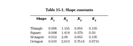
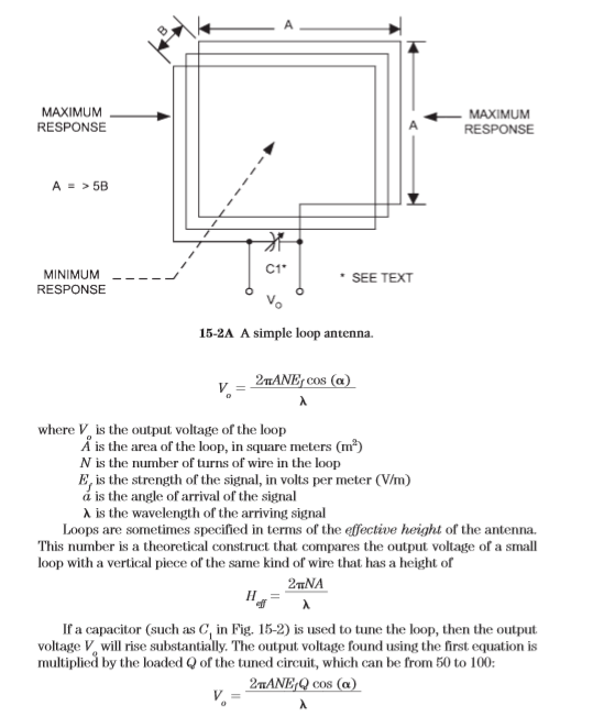
 The differences between small loops and large loops show up in some interesting ways, but perhaps the most striking is the directions of maximum response—the main lobes—and the directions of the nulls. 

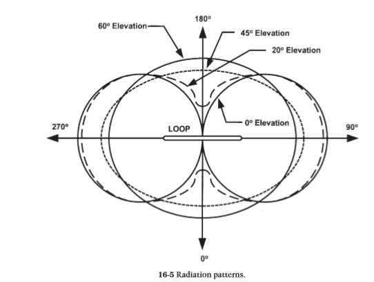
Both types of loops produce figure-8 patterns but in directions at right angles with respect to each other. The large loop antenna produces main lobes orthogonal,at right angles or “broadside,” to the plane of the loop. Nulls are off the sides of the loop. 

The small loop, however, is exactly the opposite: The main lobes are off the sides of the loop (in the direction of the loop plane), and the nulls are broadside to the loop plane (Fig. 15-1A). Do not confuse small loop behavior with the behavior of the loopstick antenna. 

Loopstick antennas are made of coils of wire wound on a ferrite or powdered-iron rod. The direction of maximum response for the loopstick antenna is broadside to the rod, with deep nulls off the ends (Fig. 15-1B). Both loopsticks and small wire loops are used for radio direction-finding and for shortwave, low-frequency medium-wave, AM broadcast band, and VLF listening.


The nulls of a loop antenna are very sharp and very deep. Small changes of pointing direction can make a profound difference in the response of the antenna. If you point a loop antenna so that its null is aimed at a strong station, the signal strength of the station appears to drop dramatically at the center of the notch. 

Turn the antenna only a few degrees one way or the other, however, and the signal strength increases sharply. The depth of the null can reach 10 to 15 dB on sloppy loops and 30 to 40 dB on well-built loops (30 dB is a very common value). I have seen claims of 60-dB nulls for some commercially available loop antennas. 

The construction and uniformity of the loop are primary factors in the sharpness and depth of the null.


At one time, the principal use of the small loop antenna was radio direction-finding, especially in the lower-frequency bands. The RDF loop is mounted with a compass rose to allow the operator to find the direction of minimum response. The null was used, rather than the peak response point, because it is far narrower than the peak. 

As a result, precise determination of direction is possible. Because the null is bidirectional, ambiguity exists as to which of the two directions is the correct direction. What the direction-finder “finds” is a line along which the station exists. If the line is found from two reasonably separated locations and the lines of direction are plotted on a map, then the two lines will cross in the area of the station. Three or more lines of direction (a process called triangulation) yields a pretty precise knowledge of the station’s actual location. 

Today, these small loops are still used for radio direction-finding, but their use has been extended into the general receiving arena, especially on the low frequencies. One of the characteristics of these bands is the possibility of strong local interference smothering weaker ground-wave and sky-wave stations.

 As a result, you cannot hear cochannel signals when one of them is very strong and the other is weak. Similarly, if a cochannel station has a signal strength that is an appreciable fraction of the desired signal and is slightly different in frequency, then the two signals will heterodyne together and form a whistling sound in the receiver output. 

The frequency of the whistle is an audio tone equal to the difference in frequency between the two signals. This is often the case when trying to hear foreign BCB signals on frequencies (called split frequencies) between the standard spacing. The directional characteristics of the loop can help if the loop null is placed in the direction of the undesired signal. 

Loops are used mainly in the low-frequency bands even though such loops are either physically larger than high-frequency loops or require more turns of wire. Loops have been used as high as VHF and are commonly used in the 10-m ham band for such activities as hidden transmitter hunts. 

The reason why low frequencies are the general preserve of loops is that these frequencies are more likely to have substantial ground-wave signals. Sky-wave signals lose some of their apparent directivity because of multiple reflections. 

Similarly, VHF and UHF waves are likely to reflect from buildings and hillsides and so will arrive at angles other than the direction of the transmitter. As a result, the loop is less useful for the purpose of radio directionfinding.

 If your goal is not RDF but listening to the station, this is hardly a problem. A small loop can be used in the upper shortwave bands to null a strong local groundwave station in order to hear a weaker sky-wave station. 

Finally, loops can be useful in rejecting noise from local sources, such as a “leaky” electric power line or a neighbor’s outdoor light dimmer. Let’s examine the basic theory of small loop antennas and then take a look at some practical construction methods.


Grover’s equation 

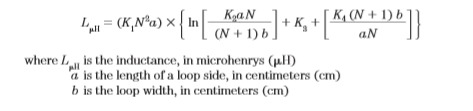
Grover’s equation (Grover, 1946) seems closer to the actual inductance measured in empirical tests than certain other equations that are in use. This equation is
n is the number of turns in the loop
K1through K4 are shape constants and are given in Table 15-1
ln is the natural log of this portion of the equation


Half Delta Sloper (HDS) Antenna

The half-delta sloper (HDS) antenna (Fig. 14-9) is similar to the full delta loop, except that (like the quarter-wavelength vertical) half of the antenna is in the form of an “image” in the ground. Gains of 1.5 to 2 dB are achievable. The HDS antenna consists of two elements: a /3-wavelength sloping wire and a /6 vertical wire (on an insulated mast), or a /6 metal mast. 

Because the ground currents are very important, much like the vertical antenna, either an extensive radial system at both ends is needed, or a base ground return wire (buried) must be provided. The HDS will work on its design frequency, plus harmonics of the design frequency. For a fundamental frequency of 5 MHz, a vertical segment of 33 ft and a sloping section of 66 ft is needed. The lengths for any frequency are found from


The HDS is fed at one corner, close to the ground. If only the fundamental frequency is desired, then you can feed it with 52-Ω coaxial cable. But at harmonics, the feedpoint impedance changes to as high as 1000 Ω. If harmonic operation is intended, then an antenna tuning unit (ATU) is needed at point A to match these impedances.

Bisquare Loop Antenna

The bisquare antenna -  The bisquare antenna offers as much as 4-dB gain broadside to the plane of the antenna (i.e., in and out of the book page), in a figure-8 pattern, on the design frequency. It is horizontally polarized. When the frequency drops to one-half of the design frequency, the gain drops to about 2 dB, and the antenna works like the diamond loop covered previously.shown in Fig. 14-10, is similar to the other large loops, except that it is /2 on each side, making a total wire length of two wavelengths. This antenna is built like the diamond loop shown earlier (i.e., it is a large square loop fed at an apex that is set at the bottom of the assembly). In this case, the loop is fed either with an antenna tuning unit (to match a 1000-Ωimpedance) or a quarter-wavelength matching section made of 300-Ω or 450-Ω twin-lead transmission line. A 1:1 balun transformer connects the 75-Ω coaxial cable to the matching section. the bi-square is not quite a real loop since it is split at the top.

The bi-square antenna offers as much as 4-dB gain broadside to the plane of the antenna (i.e., in and out of the book page), in a figure-8 pattern, on the design frequency. It is horizontally polarized. When the frequency drops to one-half of the design frequency, the gain drops to about 2 dB, and the antenna works like the diamond loop covered previously.
For bi-square Antenna many prefer use coaxial cable to the 300 ohm ribbon feedline to the bi-square normally uses.


If you think a single element quad loop (1 wavelength perimeter) is large, double its size to get an idea of the bi-square's dimensions.  But despite what it looks like from a far, the bi-square is not quite a real loop since it is split at the top.

Still, if you have one tall tower (at least 3/4 wavelength high) the bi-square may be worth considering. It's basically a bidirectional gain antenna. If you've already got the wire the construction cost is low. And you may be able to use some ingenious remote switching with relays to change the antenna into a large loop for other bands. 

1/4 Lambda Bi-Square Antenna

Another example project The Bi-Square antenna with four half-waves in phase, which makes it three half-waves and about 4 db better than dipole. The Bi-square to be described  is for 15 meters , also success used for 20m and 40m band.
The advantages of this antenna are many. It's cheap , you need only one pole, 35 feet or over, to hang it on. It is bi-directional . you can hang two of them on one pole and cover 360 degrees. It's easy to tune. It has 4 dB Gain, which puts it in the well tuned two-element beam class. It is also good competition for the "pre-tuned" or untuned three-element beam. This Bi-square antenna can feed in to 150 watt Sideband Transmitter.

Reference : Practical Antenna handbook - Joseph J. Carr
                    Antenna Magazine

Delta loop Antenna

The delta loop antenna, like the Greek uppercase letter “delta” (∆) from which it draws its name, is triangle-shaped (Fig. 14-8). The delta loop is a full wavelength, with elements approximately 2 percent longer than the natural wavelength (like the quad). The actual length will be a function of the proximity and nature of the underlying ground, so some experimentation is necessary. The approximate preadjustment lengths of the sides are found from:


The delta loop antenna is fed from 52-Ωcoaxial cable through a 4:1 balun transformer. The delta loop can be built in a fixed location, and will offer a bidirectional pattern.

Reference : Practical Antenna Handbook - by Joseph J. Carr

Demiquad Loop Antenna

The demiquad is a single-element 1 quad antenna. The length of the antenna is, like the cubical quad beam antenna (see Chap. 12), one wavelength. Figure 14-7 shows a type of demi-quad based on the tee-cross type of mast. The impedance-matching section is a quarter-wavelength piece of 75-Ω coaxial cable (RG-58/U or RF-11/U). The length of the matching section is determined from:


1 Lambda Large Loops

If size is not forcing you to a /2 loop, then a 1 loop might be just the ticket. It produces a gain of about
2 dB over a dipole in the directions that are perpendicular to the plane of the loop. The azimuth patterns formed by these antennas are similar to the figure-8 pattern of the dipole. Three versions are shown: the square loop (Fig. 14-3), the diamond loop (Fig. 14-4), and the delta loop (a.k.a. D-loop and triangle—Fig. 14-5). The square and diamond loops are built with /4 on each side, and the delta loop is /3 on each side. The overall length of wire needed to build these antennas is


The polarization of the three loop antennas is horizontal, because of the location of the feedpoints. On the square loop, moving the feedpoint to the middle of either vertical side will provide vertical polarization. Similarly, on the diamond loop vertical polarization is realized by moving the feedpoint to either of the two adjacent apexes. On the delta loop, placing the feedpoint at either of the two other apexes produces a diagonal polarization that offers approximately equal vertical and horizontal polarization components.

The feedpoint impedance of the 1 loop is around 100 Ω, so it provides a slight mismatch to 75-Ωcoax and a 2:1 mismatch to 52-Ωcoax. A very good match to 52-Ω coax can be produced using the scheme of Fig. 14-6. Here, a quarter-wavelength coaxial cable matching section is made of 75-Ω coaxial cable. The length of this cable should be

From Book : Practical Antenna Handbook - By Joseph J. Carr